提升 CUDA 内核效率与算术强度
Chapter 9. Increasing CUDA Kernel Efficiency and Arithmetic Intensity
本章目录
Even if you fully hide latency with massive parallelism and high ILP, a kernel’s performance may still be limited by how much useful work it does per memory access. Arithmetic intensity, also called operational intensity, measures how many floating-point operations are performed per byte of data transferred from memory, or FLOPS per byte.即使你通过大规模并行和高 ILP 完全隐藏了时延,内核的性能仍可能受限于它在每次显存访问中完成的有效工作量。算术强度,也称为*运算强度*,衡量的是每从内存传输一字节数据所执行的浮点运算数量,即每字节的 FLOPS。
Newer GPU generations are advancing compute throughput well beyond memory bandwidth. This widening gap means that increasing arithmetic intensity is even more critical than ever. Higher arithmetic intensity indicates a kernel does more computation for each byte fetched, which is essential for fully utilizing the GPU’s computational capabilities.新一代 GPU 的计算吞吐量提升幅度远超显存带宽。这一不断扩大的差距意味着,提升算术强度比以往任何时候都更加关键。更高的算术强度表明内核每取一字节数据就完成更多计算,这对于充分利用 GPU 的计算能力至关重要。
Arithmetic intensity is a key metric in the Roofline performance model. The Roofline model is a useful visual tool that plots kernel performance (FLOPs/sec) against arithmetic intensity (FLOPs/byte). It shows hardware ceilings (roofs) for memory bandwidth and compute throughput, allowing us to see if a kernel is memory bound, performance limited by memory transfers, or compute bound, performance limited by ALU throughput.算术强度是屋顶线模型中的关键指标。屋顶线模型是一种实用的可视化工具,它将内核性能(FLOPs/秒)对算术强度(FLOPs/字节)作图。它展示了显存带宽与计算吞吐量的硬件上限(屋顶),使我们能够判断内核是显存受限(性能受限于内存传输),还是计算受限(性能受限于 ALU 吞吐量)。
In practice, you can generate roofline charts using tools like Nsight Compute, which includes a Roofline analysis view. Using these tools, you can verify if your kernel is initially memory bound or compute bound—then continue to profile and verify improvements as you make optimizations.在实践中,你可以使用 Nsight Compute 等工具生成屋顶线图,其中包含 Roofline 分析视图。借助这些工具,你可以确认内核最初是显存受限还是计算受限,然后在进行优化时持续剖析并验证改进效果。
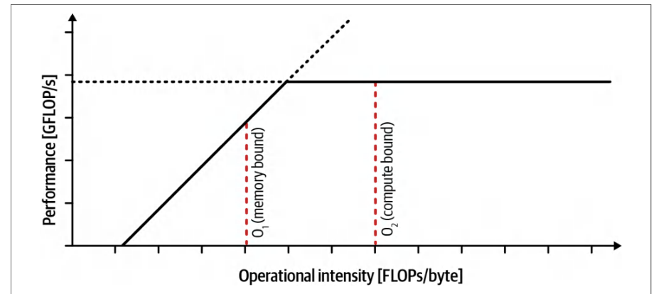
The goal is to push the kernel toward the compute-bound regime and leverage the GPUs increasing computational power. A Roofline performance model can properly guide your optimizations toward that goal.目标是推动内核进入计算受限区间,并充分利用 GPU 不断增强的计算能力。屋顶线性能模型能够正确引导你的优化朝着这一目标前进。
As shown in a previous chapter, a roofline chart uses one horizontal line to represent the hardware’s peak compute throughput (the roof)—and a diagonal line from the origin represents the peak achievable throughput limited by memory bandwidth. A kernel’s arithmetic intensity determines where it falls on the x-axis, and its performance can be compared against these ceilings, as shown in Figure 9-1.如前文某一章所示,屋顶线图用一条水平线表示硬件的峰值计算吞吐量(屋顶),用一条从原点出发的斜线表示受显存带宽限制的可达峰值吞吐量。内核的算术强度决定其在 x 轴上的位置,其性能可与这些上限进行比较,如图 9-1 所示。
A kernel with low arithmetic intensity, or few math operations per byte of data moved, will be memory bound. In this case, the kernel’s speed is capped by the hardware’s memory bandwidth, because the GPU spends most of its time waiting for data rather than crunching numbers.算术强度低(即每移动一字节数据只做很少的数学运算)的内核将是显存受限的。在这种情况下,内核的速度受硬件显存带宽的限制,因为 GPU 大部分时间都在等待数据,而不是进行数值计算。
Conversely, a kernel with very high arithmetic intensity, or many FLOPs per byte moved, will be compute bound because it is utilizing the ALUs and Tensor Cores near their peak capabilities. In this case, the kernel’s memory bandwidth usage is a secondary concern.相反,算术强度很高(即每移动一字节数据做大量 FLOPs)的内核将是计算受限的,因为它使 ALU 和张量核心接近其峰值能力运行。在这种情况下,内核的显存带宽使用量是次要考虑因素。
The goal is always to increase arithmetic intensity where possible by doing more computational work for each byte of data transferred to and from global memory (FLOPs per byte). You can increase arithmetic intensity using techniques like loop tiling to reuse data, using on-chip L1/shared memory for reuse, and fusing multiple kernels into one so that intermediate results don’t get written to global memory.目标始终是在可能的情况下提高算术强度,即对往返全局内存的每一字节数据做更多计算工作(每字节的 FLOPs)。你可以使用循环分块(loop tiling)来复用数据、利用片上 L1/共享内存进行复用,以及将多个内核融合为一个以避免中间结果写入全局内存,从而提高算术强度。
You can also use lower-precision data types (FP16, FP8, FP4) to reduce the amount of memory transfers—and utilize Tensor Cores to increase FLOPs per second. Together, these will increase the FLOPs per byte ratio and increase arithmetic intensity. Next, let’s discuss some of these techniques.你还可以使用更低精度的数据类型(FP16、FP8、FP4)来减少内存传输量,并利用张量核心提高每秒 FLOPs。两者结合将提高每字节 FLOPs 的比值,从而提升算术强度。接下来,我们讨论其中一些技术。
Keep in mind that not every workload can easily increase its arithmetic intensity. It’s constrained by algorithm characteristics. However, you should look for any opportunity to improve the algorithm, reuse data, fuse operations, and increase batch sizes to raise arithmetic intensity without changing the algorithm’s result (e.g., accuracy).请记住,并非每种工作负载都能轻易提高其算术强度。它受算法特性的约束。不过,你应当寻找任何机会来改进算法、复用数据、融合操作并增大批大小,从而在不改变算法结果(例如精度)的前提下提高算术强度。
多级微瓦片化与软件预取
Multilevel Microtiling and Software Prefetching
As discussed in Chapter 7, tiling (aka chunking or blocking) and data reuse are an effective way to raise arithmetic intensity. In that chapter, we showed how loading a small submatrix (tile) of A and B into shared memory lets each byte fetched from global memory be used for many multiply-accumulate operations at static random-access memory (SRAM) speed.如第 7 章所述,瓦片化(tiling,又称*分块*或*阻塞*)与数据复用是提高算术强度的有效方式。在该章中,我们展示了如何将 A 和 B 的一个小子矩阵(瓦片)加载到共享内存,使从全局内存取出的每个字节都能以静态随机存取存储器(SRAM)的速度参与大量乘累加运算。
Whenever you restructure code so that each element is loaded once and used tens or hundreds of times, like in the case of tiling, you multiply your FLOPs per byte ratio by the reuse factor. For instance, in a typical matrix multiply, a 32 × 32 tile of A and B produces 1,024 (1,024 = 32 × 32) independent multiplies for each element in shared memory. As such, the arithmetic intensity rises compared to fetching each element directly from DRAM for every operation.每当你重构代码,使每个元素只加载一次却被使用数十或数百次——就像瓦片化那样——你就把每字节 FLOPs 比值乘以了复用因子。例如,在典型的矩阵乘法中,A 和 B 的 32 × 32 瓦片会为共享内存中的每个元素产生 1,024(1,024 = 32 × 32)次独立乘法。因此,与每次运算都直接从 DRAM 取每个元素相比,算术强度得以提升。
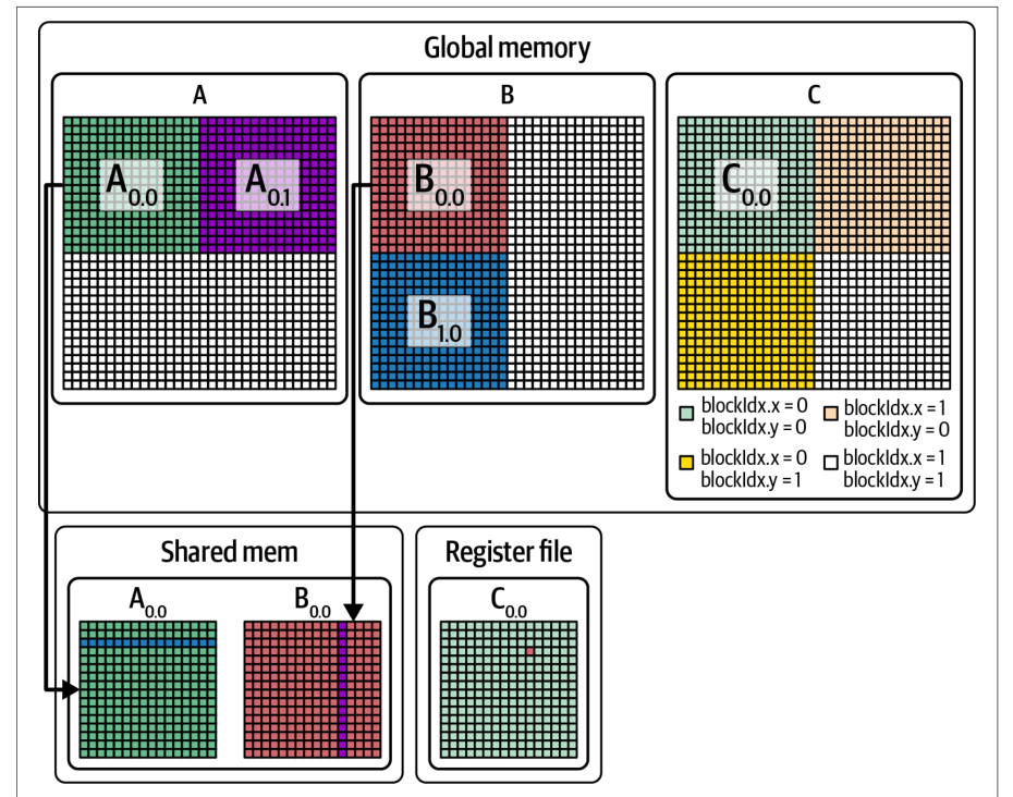
Beyond simple shared-memory tiling, you can further increase intensity and expose more ILP with multilevel tiling. With multilevel tiling, after staging a tile into shared memory, you have each thread load microtiles into registers using vectorized types such as float4 and <half2>. This way, repeated operations happen entirely in registers. An example of multilevel tiling is shown in Figure 9-2.除了简单的共享内存瓦片化之外,你还可以通过多级瓦片化进一步提高强度并暴露更多指令级并行(ILP)。在多级瓦片化中,将瓦片暂存到共享内存后,让每个线程使用 float4、<half2> 等向量化类型把微瓦片加载到寄存器。这样,重复的运算完全在寄存器中进行。图 9-2 给出了多级瓦片化的一个示例。
This intra-SM reuse (register → SMEM → DRAM) reduces the working set at every level—and minimizes off-chip traffic. As always, be sure to coalesce global reads when filling shared memory and pad/swizzle shared data to avoid memory-bank conflicts, as we covered in Chapter 7.这种 SM 内复用(寄存器 → SMEM → DRAM)在每一层级都缩小了工作集,并最大限度地减少了片外流量。一如既往,在填充共享内存时务必对全局读取做合并访问,并对共享数据做填充/重排(swizzle)以避免存储体冲突,正如第 7 章所述。
On modern GPUs, these inner-loop tiling steps are often covered by using MMA fragment APIs. The hardware moves data between shared memory and Tensor Memory (TMEM) implicitly using Tensor Core instructions. TMEM usage is managed by the compiler and libraries. On modern GPUs, tcgen05 instructions implicitly stage data between shared memory and TMEM. They use a distinct TMEM address space. However, developers can still manually move tiles into shared memory with cp.async or TMA when implementing certain algorithms and need explicit control.在现代 GPU 上,这些内层循环的瓦片化步骤通常由 MMA 片段 API 覆盖。硬件使用张量核心指令在共享内存与张量内存(TMEM)之间隐式搬运数据。TMEM 的使用由编译器和库管理。在现代 GPU 上,tcgen05 指令在共享内存与 TMEM 之间隐式暂存数据。它们使用独立的 TMEM 地址空间。不过,在实现某些算法并需要显式控制时,开发者仍可以用 cp.async 或 TMA 手动将瓦片搬入共享内存。
A closely related technique is software prefetching, which is often implemented as double buffering. For instance, instead of waiting until the current tile’s computations finish, you can issue asynchronous loads for the next tile into shared memory. This will overlap DRAM → shared-memory (SMEM) transfers with ongoing arithmetic. Careful prefetching can significantly reduce stall time and improve throughput. The idea is to overlap data transfer with computation so the ALUs never starve waiting for data.一项密切相关的技术是软件预取,它通常以双缓冲的形式实现。例如,不必等到当前瓦片的计算完成,你就可以为下一个瓦片向共享内存发起异步加载。这会让 DRAM → 共享内存(SMEM)的传输与正在进行的算术运算重叠。精心的预取可以显著减少停顿时间并提升吞吐量。其思路是让数据传输与计算重叠,使 ALU 永远不会因等待数据而空转。
When using unified memory with a CPU-GPU superchip like Grace Blackwell, you can use cudaMemPrefetchAsync() to hint that a tile will be needed soon. This hints at the runtime to migrate pages over NVLink-C2C. However, prefetch is just a hint and not a guarantee. You still want to make sure you are overlapping transfers and synchronizing appropriately to avoid page fault stalls. Overlapping data movement with compute in this way ensures the ALUs remain fed whenever a new tile is needed. This further hides memory latency—and boosts achieved FLOPS.在 Grace Blackwell 这类 CPU-GPU 超级芯片上使用统一内存时,你可以用 cudaMemPrefetchAsync() 提示某个瓦片很快会被用到。这会向运行时提示通过 NVLink-C2C 迁移页面。然而,预取只是一个提示,并非保证。你仍需确保传输相互重叠并恰当地同步,以避免缺页停顿。以这种方式让数据搬运与计算重叠,可确保在需要新瓦片时 ALU 始终有数据可用。这进一步隐藏了内存时延,并提升了实际达到的 FLOPS。
In short, the more times that each byte from DRAM is reused at the on-chip levels (registers or shared memory), the higher your arithmetic intensity. And higher arithmetic intensity moves the kernel closer into the compute-bound regime.简而言之,DRAM 中的每个字节在片上层级(寄存器或共享内存)被复用的次数越多,算术强度就越高。而算术强度越高,内核就越接近计算受限(compute-bound)区间。
使用线程块集群进行分块
Tiling with Thread Block Clusters
On modern GPUs, you can extend the tiling-reuse idea using CUDA thread-block clusters from Cooperative Groups (discussed in Chapter 10). These allow multiple thread blocks to share data using distributed shared memory (DSMEM), as shown in在现代 GPU 上,可以使用 Cooperative Groups 提供的 CUDA 线程块集群(thread block cluster)来扩展分块复用的思路(第 10 章将讨论)。这些集群允许多个线程块通过分布式共享内存(DSMEM)共享数据,如图所示
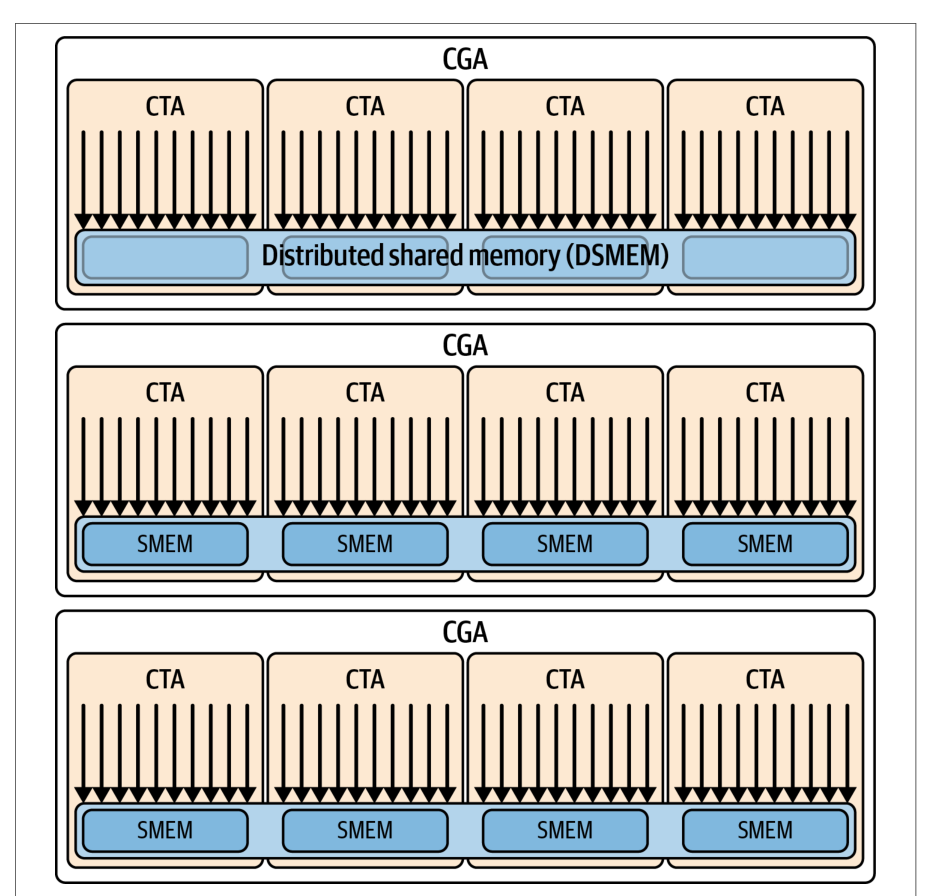
We cover CGAs and thread block clusters in detail in the next chapter, but they’re worth mentioning here, as they can directly increase arithmetic intensity. For example, a cluster of four thread blocks can cooperatively load one tile using the Tensor Memory Accelerator (TMA) multicast feature, as shown in Figure 9-4, which uses four CTAs to demonstrate this mechanism.我们将在下一章详细讨论 CGA 和线程块集群,但这里值得一提,因为它们可以直接提高算术强度。例如,由四个线程块组成的集群可以使用张量内存加速器(TMA)的多播(multicast)特性协作加载一个分块,如图 9-4 所示,该图使用四个 CTA 来演示这一机制。
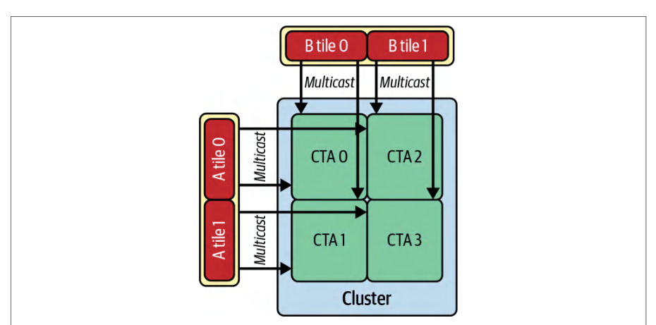
Each tile is partitioned across the four thread blocks so that global memory traffic for that tile is amortized over the cluster. The tiles are fetched only once and reused by all four thread blocks.每个分块被划分到四个线程块上,从而使该分块的全局内存流量在整个集群上分摊。分块只被取一次,并由全部四个线程块复用。
Thread block clusters can reduce global memory traffic by up to 4× in a 2 × 2 cluster when four CTAs reuse the same data using multicast. Also, thread block clusters increase arithmetic intensity per GPU by lowering the denominator, or number of bytes moved from global memory. A specialized form of these called thread block pairs will be discussed in a bit—in the context of tiling with Tensor Cores.当四个 CTA 使用多播复用同一份数据时,线程块集群在 2 × 2 集群中最多可将全局内存流量降低 4 倍。此外,线程块集群通过降低分母,即从全局内存搬运的字节数,来提高每块 GPU 的算术强度。其中一种特殊形式称为*线程块对*(thread block pair),稍后将在使用张量核心进行分块的语境下讨论。
内核融合
Kernel Fusion
Another way to increase arithmetic intensity is to fuse multiple operations—or loop iterations—into one operation. By fusing together multiple kernels, the data loaded from memory can be used for several computations and iterations before being written back.提高算术强度的另一种方式是将多个操作(或循环迭代)融合为一个操作。通过将多个内核融合在一起,从内存加载的数据可以在写回之前用于多次计算和迭代。
Similarly, loop unrolling, discussed in the previous section, allows a single thread to perform more calculations on each loaded data element, but at the cost of more register usage. Too much fusion can increase per-thread register pressure and reduce occupancy, so there’s a trade-off.类似地,上一节讨论的循环展开允许单个线程对每个已加载的数据元素执行更多计算,但代价是占用更多寄存器。过度融合会增加每线程的寄存器压力并降低占用率,因此存在权衡。
Always profile fused kernels. If register usage becomes excessive and starts spilling to local memory, the benefits of fusion might be offset by the additional memory traffic. If you find the right balance, however, you can improve the FLOPS per byte moved, and this is beneficial if memory bandwidth is a limiting factor.务必对融合后的内核做性能剖析。如果寄存器用量过大并开始溢出到本地内存,融合带来的收益可能被额外的内存流量抵消。不过,如果找到合适的平衡点,就能提高每搬运一个字节所获得的 FLOPS,这在显存带宽成为限制因素时是有益的。
Modern deep learning frameworks can automatically fuse and unroll through their just-in-time compilers and graph optimizers. For instance, PyTorch’s torch.compile, and specifically TorchInductor, can automatically fuse sequences of elementwise operations. We cover the PyTorch compiler in Chapters 13 and 14.现代深度学习框架可以通过其即时编译器和图优化器自动完成融合与展开。例如,PyTorch 的 torch.compile,特别是 TorchInductor,可以自动融合一连串逐元素操作。我们将在第 13 章和第 14 章介绍 PyTorch 编译器。
Fusing these elementwise operations eliminates unnecessary memory traffic by keeping intermediate values on-chip. This increases the amount of work done per byte fetched from global memory—raising the arithmetic intensity.融合这些逐元素操作可以把中间值保留在片上,从而消除不必要的内存流量。这提高了每从全局内存取一个字节所完成的工作量——即提升了算术强度。
For instance, the naive implementation launches two kernels. The first kernel reads x and writes y to global memory. The second reads y and writes z:例如,朴素实现会启动两个内核。第一个内核读取 x 并将 y 写入全局内存。第二个内核读取 y 并写入 z:
y = sin(x);
z = sqrt(y);
Here, each element is touched twice: once after sin(x) and once after sqrt(y). As such, each kernel’s arithmetic intensity is very low, since it performs just one expensive math function (a multicycle ALU instruction) per element—per load/store operation. In contrast, the fused kernel performs this same set of operations in a single pass:这里,每个元素被访问两次:一次在 sin(x) 之后,一次在 sqrt(y) 之后。因此,每个内核的算术强度都非常低,因为它对每个元素——即每次加载/存储操作——只执行一个开销较大的数学函数(一条多周期 ALU 指令)。相比之下,融合后的内核在单次遍历中完成同一组操作:
z[i] = sqrt(sin(x[i]));
Each x[i] is loaded once, then both sin and sqrt are applied in registers, and only the final z[i] is written to memory. Because the intermediate y never goes out to global memory, the effective FLOPS per byte jump sharply, moving the operation closer to the compute roof.每个 x[i] 只加载一次,随后 sin 和 sqrt 都在寄存器中执行,只有最终的 z[i] 被写入内存。由于中间结果 y 从不写入全局内存,每字节的有效 FLOPS 急剧上升,使该操作更接近计算屋顶。
Fusion reduces global memory traffic and increases arithmetic intensity since each element now undergoes two math operations for each read and write memory operation. In our example, we doubled the FLOPS per element (sin + sqrt) while roughly halving the memory traffic since there is no intermediate write. This produces a significantly higher arithmetic intensity, or FLOPS/byte.融合减少了全局内存流量并提高了算术强度,因为现在每个元素在每次读、写内存操作中都要经历两次数学运算。在我们的示例中,每个元素的 FLOPS 翻倍(sin + sqrt),而由于没有中间写入,内存流量大约减半。这带来了显著更高的算术强度,即 FLOPS/字节。
To drive this point home, let’s demonstrate arithmetic intensity with a concrete example. Suppose we want to L2-normalize each length-hidden row of a 2D tensor x (shape [batch, hidden]). For each row b, compute a single norm, norm_b = sqrt(Σ_i x[b,i]*x[b,i] + ε), and then write y[b,i] = x[b,i] / norm_b for all i.为了把这一点讲透彻,我们用一个具体例子来演示算术强度。假设我们要对一个二维张量 x(形状为 [batch, hidden])中每一行长度为 hidden 的行做 L2 归一化。对每一行 b,先计算一个范数 norm_b = sqrt(Σ_i x[b,i]*x[b,i] + ε),然后对所有 i 写入 y[b,i] = x[b,i] / norm_b。
A naive implementation would square in one kernel, reduce each row to a scalar in a second kernel, and divide in a third kernel. This would require multiple kernel launches with intermediate writes to HBM.朴素实现会在一个内核中做平方,在第二个内核中把每一行归约为一个标量,在第三个内核中做除法。这需要多次内核启动,并向 HBM 写入中间结果。
Let’s assume that each of the 4 kernels requires 1 FLOP of compute. As such, the arithmetic intensity of each of the 4 kernels is 1 FLOP per 12 bytes (2 float reads, 1 float write), or 0.083 FLOPS/byte.假设这 4 个内核每个都需要 1 FLOP 的计算量。因此,4 个内核各自的算术强度都是每 12 字节 1 FLOP(2 次 float 读、1 次 float 写),即 0.083 FLOPS/字节。
Instead, we can fuse the 4 kernels into a single kernel and increase the arithmetic intensity. The manually fused kernel code is shown here:取而代之,我们可以把这 4 个内核融合为单个内核,从而提高算术强度。手动融合后的内核代码如下:
__global__ void fusedL2Norm(const float* __restrict__ x,
                            float* __restrict__ y,
                            int hidden) {
  extern __shared__ float sdata[];        // 归约缓冲区
  const int batch   = blockIdx.x;         // 每个批次行一个线程块
  const int tid     = threadIdx.x;
  const float* batch_ptr = x + size_t(batch) * hidden;
  // 1) 将平方和累加到共享内存
  float local = 0.f;
  for (int i = tid; i < hidden; i += blockDim.x) {
    float v = batch_ptr[i];
    local   = fmaf(v, v, local);          // v*v + local
  }
  sdata[tid] = local;
__global__ void fusedL2Norm(const float* __restrict__ x,
                            float* __restrict__ y,
                            int hidden) {
  extern __shared__ float sdata[];        // reduction buffer
  const int batch   = blockIdx.x;         // one block per batch row
  const int tid     = threadIdx.x;
  const float* batch_ptr = x + size_t(batch) * hidden;
  // 1) Accumulate sum of squares into shared memory
  float local = 0.f;
  for (int i = tid; i < hidden; i += blockDim.x) {
    float v = batch_ptr[i];
    local   = fmaf(v, v, local);          // v*v + local
  }
  sdata[tid] = local;
  __syncthreads();
  // 2) 并行归约到 sdata[0]
  for (int offset = blockDim.x >> 1; offset > 0; offset >>= 1) {
    if (tid < offset) sdata[tid] += sdata[tid + offset];
    __syncthreads();
  }
  // 3) 归一化(防范过小的范数)
  float norm = sqrtf(sdata[0]);
  float inv = rsqrtf(sdata[0]); // 优先使用倒数
  float* out_batch = y + size_t(batch) * hidden;
  for (int i = tid; i < hidden; i += blockDim.x) {
    // 乘以倒数(rsqrt)与除以 sqrt 的对比
    out_batch[i] = batch_ptr[i] * inv;
  }
}
  __syncthreads();
  // 2) Parallel reduction to sdata[0]
  for (int offset = blockDim.x >> 1; offset > 0; offset >>= 1) {
    if (tid < offset) sdata[tid] += sdata[tid + offset];
    __syncthreads();
  }
  // 3) Normalize (guard tiny norms)
  float norm = sqrtf(sdata[0]);
  float inv = rsqrtf(sdata[0]); // prefer inverse
  float* out_batch = y + size_t(batch) * hidden;
  for (int i = tid; i < hidden; i += blockDim.x) {
    // multiply by inverse (rsqrt) vs. divide by sqrt
    out_batch[i] = batch_ptr[i] * inv;
  }
}
In this fused kernel, each thread walks its slice of x[b,*] twice—once to accumulate a local sum of squares and once to write the normalized outputs—so global traffic is ~12 bytes per element (two reads + one write). Per element the kernel does ~1 multiply + 1 add during the reduction and 1 multiply during the normalize.在这个融合内核中,每个线程两次遍历自己负责的 x[b,*] 片段——一次累加局部平方和,一次写出归一化结果——因此每个元素的全局流量约为 12 字节(两次读 + 一次写)。对每个元素,内核在归约阶段约做 1 次乘法 + 1 次加法,在归一化阶段做 1 次乘法。
The sqrt and rsqrt are amortized over the whole row. For roofline placement, a conservative arithmetic intensity is ≈3 FLOPs / 12 bytes ≈ 0.25 FLOPs/byte (plus the tiny 1/(hidden * 12) contribution from the per-row sqrt). This lets us hide sqrt and rsqrt latency by giving each thread multiple elements to increase ILP.sqrt 和 rsqrt 的开销被摊到整行上。就屋顶线模型定位而言,保守的算术强度约为 ≈3 FLOPs / 12 字节 ≈ 0.25 FLOPs/字节(再加上每行 sqrt 带来的极小贡献 1/(hidden * 12))。这让我们可以通过给每个线程分配多个元素来提高 ILP,从而隐藏 sqrt 和 rsqrt 的时延。
Compared to a naive three-kernel pipeline (square → reduce → divide) with intermediate writes to HBM, the fused version removes at least one global write/read round trip and one launch barrier. As such, its intensity and runtime are much better in practice—even though the per-element FLOP/byte is only ~0.25. This is due to latency savings and cache locality improvements.与朴素的三内核流水线(平方 → 归约 → 除法)相比——该流水线需要将中间结果写入 HBM——融合版本至少省去了一次全局写/读往返和一次启动屏障。因此,尽管每元素的 FLOP/字节仅为约 0.25,其实际算术强度和运行时间都要好得多。这得益于时延的节省和缓存局部性的改善。
In practice, this single fused kernel executes faster than a series of separate kernels due to higher arithmetic intensity (FLOPS/byte), better cache locality, and reduced launch overhead by collapsing three separate kernels into one.在实践中,这个单一融合内核比一系列独立内核执行得更快,原因在于更高的算术强度(FLOPS/字节)、更好的缓存局部性,以及将三个独立内核合并为一个所带来的启动开销降低。
Fusing not only increases arithmetic intensity and pushes the kernel more toward the compute-bound side of the roofline, but it also saves memory bandwidth. In the naive, multikernel version, we have to write intermediate results to global memory and read them back in the next kernel. In the fused version, the intermediate results (e.g., ai*ai) never have to leave the thread’s registers.融合不仅提高了算术强度、使内核在屋顶线模型上更偏向计算受限一侧,还节省了显存带宽。在朴素的多内核版本中,我们必须把中间结果写入全局内存,并在下一个内核中再读回来。而在融合版本中,中间结果(例如 ai*ai)始终无需离开线程的寄存器。
In the code example, the addition can use those registers directly to calculate the sum. The sqrt can then use the sum—all without requiring additional global memory traffic. Only the final result is written back to global memory.在代码示例中,加法可以直接使用这些寄存器来计算和。随后 sqrt 可以使用该和——全程无需额外的全局内存流量。只有最终结果被写回全局内存。
As such, the fused kernel achieves perhaps 4 FLOPS for 12 bytes of data movement from/to global memory, whereas the naive, unfused approach achieves 4 FLOPS for 36 bytes loaded and stored after accounting for the intermediate memory movement. This means less DRAM traffic and lower latency.因此,融合内核大约以 12 字节的全局内存数据搬运实现了 4 FLOPS,而朴素的非融合方法在计入中间内存搬运后,需要加载和存储 36 字节才能实现 4 FLOPS。这意味着更少的 DRAM 流量和更低的时延。
This simple example shows how fusion increases our kernel’s arithmetic intensity and overall performance. Let’s look at another way to increase arithmetic intensity by utilizing our GPUs’ Tensor Core hardware units.这个简单的例子展示了融合如何提高内核的算术强度和整体性能。接下来我们看看利用 GPU 张量核心硬件单元提高算术强度的另一种方式。
结构化稀疏性
Structured Sparsity
On modern GPUs, 2:4 structured sparsity is accelerated in hardware by Sparse Tensor Cores and cuSPARSELt. 2:4 means that exactly two out of every four consecutive weights are nonzero. Creating this type of sparsity is sometimes called pruning.在现代 GPU 上,2:4 结构化稀疏性由稀疏张量核心(Sparse Tensor Cores)和 cuSPARSELt 在硬件层面加速。2:4 意味着每四个连续权重中恰好有两个非零。创建这类稀疏性有时被称为*剪枝*。
By pruning half of the weights into a 2:4 pattern, each memory load now delivers twice as many nonzero values that actually participate in multiplication. In other words, you are no longer fetching weights that turn out to be zero. As such, you are not wasting a matrix multiply operation on something that you know is zero, as shown in Figure 9-5.通过将一半权重剪枝为 2:4 模式,每次内存加载现在能带来两倍于原来的、真正参与乘法的非零值。换言之,你不再取回那些结果为零的权重。因此,你不会把矩阵乘法运算浪费在已知为零的元素上,如图 9-5 所示。
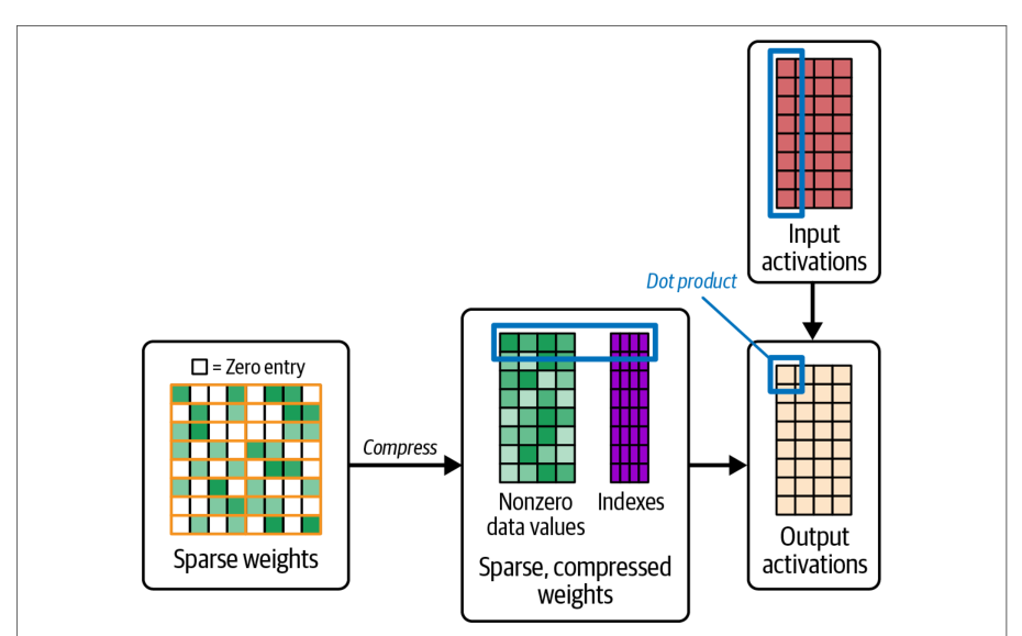
Structured sparsity is applied after a model is trained. The model is pruned and optimized for inference. Pruning and format conversion are done in software stacks such as cuSPARSELt and framework tooling. Note that the Transformer Engine accelerates supported sparse executions but does not enforce sparsity during conversion.结构化稀疏性是在模型训练完成之后应用的。模型会被剪枝并针对推理进行优化。剪枝与格式转换在 cuSPARSELt 和框架工具链等软件栈中完成。请注意,Transformer Engine 会加速受支持的稀疏执行,但在转换过程中并不强制稀疏性。
Pruning and format conversion are handled in software—typically through cuSPARSELt and framework tooling. In PyTorch, use to_sparse_semi_structured() to convert trained dense modules into 2:4 sparse format before deploying sparse GEMMs on Sparse Tensor Cores.剪枝与格式转换由软件处理——通常通过 cuSPARSELt 和框架工具链。在 PyTorch 中,使用 to_sparse_semi_structured() 将训练好的稠密模块转换为 2:4 稀疏格式,然后在稀疏张量核心上部署稀疏 GEMM。
Once your model is converted, it will invoke optimized sparse GEMM kernels running on the Sparse Tensor Cores instead of standard kernels. Sparse Tensor Cores can approach up to a 2× speedup over their dense counterparts for many inference workloads—especially when submitting large batches of inputs, as these amortize kernel launch overhead.模型转换完成后,将调用运行在稀疏张量核心上的优化稀疏 GEMM 内核,而不是标准内核。对于许多推理工作负载,稀疏张量核心相比其稠密对应实现可接近最高 2× 的加速——尤其是在提交大批量输入时,因为这样可以摊薄内核启动开销。
This gives the sparse-accelerated matrix multiplies enough parallel work to hide any overhead from handling indices or compressed representations. In smaller batches, this overhead can dominate and limit how much speedup you observe.这为稀疏加速的矩阵乘法提供了足够的并行工作,以隐藏处理索引或压缩表示带来的任何开销。在较小的批大小下,这种开销可能占据主导地位,并限制你观察到的加速幅度。
2:4 sparsity will produce maximum benefit when using large matrix multiplies, which are common in transformer-based models like LLMs. This is because the hardware can fully utilize the dedicated Sparse Tensor Cores. These Sparse Tensor Cores operate on half-width data directly in hardware. This skips zeros and performs twice the work on the nonzero elements in the same cycle budget.2:4 稀疏性在使用大矩阵乘法时收益最大,而这在 LLM 等基于 Transformer 的模型中很常见。这是因为硬件可以充分利用专用的稀疏张量核心。这些稀疏张量核心直接在硬件层面处理半宽数据。它跳过零元素,并在相同的周期预算内对非零元素执行两倍的工作。
Because compute capacity on Blackwell has grown faster than HBM bandwidth, structured sparsity is a great way to stay compute bound. Even on a Grace Blackwell system in which NVLink-C2C lets the GPU stream data from CPU memory at very high throughput, you still want to maximize FLOPS per byte on every loaded tile.由于 Blackwell 上的计算能力增长快于 HBM 带宽,结构化稀疏性是保持计算受限的绝佳方式。即使在 Grace Blackwell 系统上,NVLink-C2C 让 GPU 能以极高吞吐量从 CPU 内存流式读取数据,你仍然希望最大化每个加载瓦片(tile)的每字节 FLOPS。
By pruning 50% of weights in a 2:4 pattern, for instance, you ensure that half of your memory traffic is never needed. This immediately reduces global-memory reads and raises effective arithmetic intensity by almost 2×.例如,以 2:4 模式剪掉 50% 的权重,就能确保一半的内存流量根本不需要。这立即减少了全局内存读取,并将有效算术强度提高近 2×。
NVIDIA GPUs implement this 2:4 structured sparsity in hardware such that every 16-element chunk can zero out 8 elements. This is the pattern used to double Tensor Core throughput for sparse matrices. As of this writing, no other arbitrary sparsity pattern gains this special acceleration in hardware.NVIDIA GPU 在硬件中实现这种 2:4 结构化稀疏性,使得每个 16 元素块可以清零 8 个元素。正是这种模式被用来将稀疏矩阵的张量核心吞吐量翻倍。截至本文撰写时,尚无其他任意稀疏模式能在硬件中获得这种特殊加速。
Before applying sparsity, it is important to first implement the fundamental optimizations covered previously: coalesce all global loads, reuse data using tiling, and fuse pointwise operations to eliminate extra memory round trips. Once these basics are in place and verified, structured sparsity can provide another speedup for inference.在应用稀疏性之前,重要的是先实现前面介绍的基础优化:合并所有全局加载、使用分块(tiling)复用数据,并融合逐点操作以消除额外的内存往返。一旦这些基础工作到位并经过验证,结构化稀疏性可以为推理带来进一步的加速。
重计算与内存的权衡
Recomputation Versus Memory Trade-Off
Also, instead of storing or loading precomputed values (e.g., x²), consider recomputing them on demand if memory bandwidth is the bottleneck. For instance, repeatedly computing x*x in registers is often faster than loading a previously computed x² from global memory. Continuous recomputation of cheap expressions can increase arithmetic intensity and is a useful technique whenever memory is scarce.此外,如果显存带宽是瓶颈,那么与其存储或加载预先计算好的值(例如 x²),不如考虑按需重新计算它们。例如,在寄存器中反复计算 x*x 通常比从全局内存加载先前计算出的 x² 更快。对廉价表达式进行持续重算可以提高算术强度,只要内存紧张,这就是一项有用的技术。
Many LLM inference engines use this technique to save memory. Instead of storing large activation tensors in HBM and reading them back later, they can recompute certain layers and activations on the fly. This is similar to activation checkpointing in a model training context.许多 LLM 推理引擎使用这一技术来节省显存。它们不在 HBM 中存储大型激活张量并在之后读回,而是即时重算某些层和激活。这类似于模型训练场景中的*激活检查点*(activation checkpointing)。
Recomputation improves effective FLOPS/byte and can fit large models into a smaller amount of memory. In addition, recomputation frees up memory for larger batch sizes and trades a few extra FLOPS for a significant decrease in memory traffic.重算提高了有效 FLOPS/byte,并能让大型模型装入更小的内存。此外,重算为更大的批大小腾出内存,用少量额外的 FLOPS 换取内存流量的显著下降。
PyTorch 与算术强度
PyTorch and Arithmetic Intensity
In PyTorch, many of these ideas are automatically applied. As mentioned, PyTorch compiler (discussed in Chapters 13 and 14) can automatically fuse chains of elementwise operations—and even some reductions. It uses execution-graph-level optimizations to keep data on the GPU and reuse it as much as possible.在 PyTorch 中,这些想法中有许多会被自动应用。如前所述,PyTorch 编译器(在第 13 章和第 14 章讨论)可以自动融合逐元素操作的链条——甚至某些归约。它利用执行图级别的优化,将数据保留在 GPU 上并尽可能复用。
Because it uses optimized libraries like cuDNN and cuBLAS under the hood, PyTorch will perform tiling and use shared memory for you when performing matrix operations with torch.matmul. In addition, PyTorch’s scaled_dot_product_attention (SPDA) may dispatch to FlashAttention, memory-efficient, or cuDNN backends depending on tensor shapes and dtypes. To control the backend selection, use torch.nn.attention.sdpa_kernel(SDPBackend.FLASH_ATTENTION), for instance. As a performance-minded developer, you should be aware of these optimizations and how to verify when they’re being used.由于底层使用 cuDNN 和 cuBLAS 等经过优化的库,PyTorch 在用 torch.matmul 执行矩阵运算时会为你完成分块(tiling)并使用共享内存。此外,PyTorch 的 scaled_dot_product_attention(SPDA)会根据张量形状和 dtypes 分派到 FlashAttention、内存高效(memory-efficient)或 cuDNN 后端。要控制后端选择,可以使用例如 torch.nn.attention.sdpa_kernel(SDPBackend.FLASH_ATTENTION)。作为注重性能的开发者,你应当了解这些优化,以及如何验证它们何时被使用。
It’s important to note that while PyTorch can recognize and compile most operations, some nonstandard operations or custom CUDA operations might not get fused. In these cases, manual optimization may still be required, such as fusion, tiling, etc.需要注意的是,尽管 PyTorch 能够识别并编译大多数操作,某些非标准操作或自定义 CUDA 操作可能不会被融合。在这些情况下,仍可能需要手动优化,例如融合、分块等。
PyTorch’s nested tensors, or ragged tensors, let you represent batches of variable-length inputs without padding. Each nested tensor packs the variable-length sequences into a single, efficient underlying buffer. NestedTensor exposes the normal tensor interface, but it eliminates unnecessary zero-padding. As such, global-memory loads become more efficient because each byte that is fetched is useful in the computation.PyTorch 的嵌套张量(nested tensor),或称不规则张量(ragged tensor),让你无需填充即可表示变长输入的批次。每个嵌套张量将变长序列打包进单个高效的基础缓冲区。NestedTensor 暴露常规的张量接口,但消除了不必要的零填充。因此,全局内存加载变得更高效,因为取回的每个字节都在计算中有用。
Nested tensors are useful for LLMs with varying-length sequences. When using nested tensors, operations like attention and batch-matrix multiplies will retrieve only the essential data from memory. This moves your kernel closer to the compute-bound regime on the Roofline model and helps to reduce memory-bound stalls. The result is higher sustained throughput—especially on memory-sensitive workloads.嵌套张量对具有变长序列的 LLM 很有用。使用嵌套张量时,注意力和批量矩阵乘法等操作只会从内存中取回必要的数据。这使你的内核在屋顶线模型上更接近计算受限区间,并有助于减少显存受限的停顿。结果是更高的持续吞吐量——尤其是在对内存敏感的工作负载上。
In short, PyTorch exposes various mechanisms to increase your kernel’s arithmetic intensity. It’s important to understand these options and decide what works best for your workload. Another effective method to increase arithmetic intensity on modern GPUs is by using the reduced-precision Tensor Cores. Let’s cover these mechanisms next.简而言之,PyTorch 提供了多种机制来提升内核的算术强度。理解这些选项并判断哪一种最适合你的工作负载非常重要。在现代 GPU 上提升算术强度的另一种有效方法是使用低精度张量核心。接下来我们将介绍这些机制。
混合精度与张量核心的利用
Mixed Precision and Utilizing Tensor Cores
Modern NVIDIA GPUs implement reduced-precision computations like TF32, FP16, FP8, FP4, and INT8 in Tensor Cores. Each SM in Blackwell has a 256 KB on-chip TMEM dedicated to Tensor Core data. It also has a specialized TMA unit that asynchronously copies tiles between global memory and shared memory. Tensor Core instructions (e.g., tcgen05.mma) then move operands and accumulators between shared memory and TMEM implicitly. This design feeds the Tensor Cores at high throughput and minimizes stalls. Blackwell’s TMEM-based accumulators help to reduce register pressure relative to previous GPU generations which accumulated directly in registers.现代 NVIDIA GPU 在张量核心中实现 TF32、FP16、FP8、FP4 和 INT8 等低精度计算。Blackwell 的每个 SM 都有一个 256 KB 的片上 TMEM,专用于存放张量核心数据。它还有一个专用的 TMA 单元,可在全局内存与共享内存之间异步拷贝数据块(tile)。随后,张量核心指令(例如 tcgen05.mma)会隐式地在共享内存与 TMEM 之间移动操作数和累加器。这种设计以高吞吐量为张量核心供给数据,并最大限度地减少停顿。与直接在寄存器中累加的前几代 GPU 相比,Blackwell 基于 TMEM 的累加器有助于降低寄存器压力。
When used correctly, these features can transform a once memory-bound, tensor-heavy kernel into a fully compute-bound one by raising arithmetic intensity (FLOPS per byte) by 2×, 4×, or even 8×. You can verify the impact by monitoring the Roofline chart and Stall Stats in Nsight Compute.若使用得当,这些特性可将算术强度(每字节 FLOPS)提升 2 倍、4 倍甚至 8 倍,从而把一个曾经受限于内存、以张量运算为主的内核转变为完全受限于计算的内核。你可以通过观察 Nsight Compute 中的屋顶线模型图表和停顿统计(Stall Stats)来验证这一影响。
Nsight Compute’s Speed of Light analysis shows memory-bound stall reasons such as “Memory Throttle” and cache misses. These will drop significantly when usingNsight Compute 的 Speed of Light 分析会显示受限于内存的停顿原因,例如“Memory Throttle”和缓存未命中。在使用
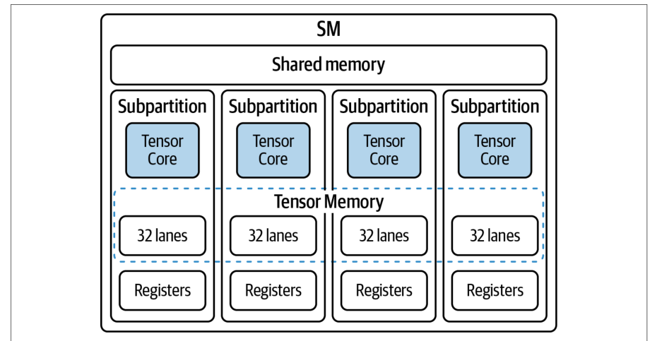
Tensor Cores with lower precision formats. And Nsight Compute integrates a Roofline chart to cross-check if arithmetic intensity increased to push your kernel toward the compute roof.低精度格式的张量核心时,这些停顿会显著减少。此外,Nsight Compute 集成了屋顶线模型图表,可用于交叉验证算术强度是否已提升,从而将你的内核推向计算屋顶。
As you move from FP32 to lower-precision Tensor Core kernels such as TF32, FP16, FP8, or FP4, Nsight Compute’s Warp Stall metrics typically show a reduction in memory-related stall as well as a relative increase in dependency or pipeline stalls. This indicates an increase in arithmetic intensity and a shift from memory-bound toward compute-bound execution.当你从 FP32 转向 TF32、FP16、FP8 或 FP4 等低精度张量核心内核时,Nsight Compute 的线程束停顿(Warp Stall)指标通常显示内存相关停顿减少,同时依赖停顿或流水线停顿相对增加。这表明算术强度提高,执行从受限于内存转向受限于计算。
使用 TMEM 和 TMA 为张量核心供给数据
Feeding Tensor Cores with TMEM and TMA
At the heart of high-throughput tensor computation is TMEM, a 256 KB SRAM buffer per SM. At a high level, programmers do not explicitly allocate or manage TMEM, however. TMEM is handled by the hardware or libraries when you use Tensor Core operations. TMEM is shown in Figure 9-6.高吞吐量张量计算的核心是 TMEM,即每个 SM 上 256 KB 的 SRAM 缓冲区。不过从高层来看,程序员并不显式分配或管理 TMEM。当你使用张量核心操作时,TMEM 由硬件或库来管理。TMEM 如图 9-6 所示。
Under the hood, Blackwell uses tcgen05.mma instructions that operate with TMEM for operand and accumulator storage. CUTLASS and library kernels manage the required allocation and usage through the kernel configuration and Parallel Thread Execution (PTX) assembly. As such, the Transformer Engine uses TMEM for partial results. This reduces the MMA dependencies on registers.在底层,Blackwell 使用 tcgen05.mma 指令,这些指令借助 TMEM 存储操作数和累加器。CUTLASS 和库内核通过内核配置和并行线程执行(PTX)汇编来管理所需的分配与使用。因此,Transformer Engine 使用 TMEM 存放部分结果。这减少了 MMA 对寄存器的依赖。
High-level APIs like CUTLASS handle all of this complexity for you automatically. Use CUTLASS and other high-level libraries when possible as CUTLASS uses the tcgen05.* PTX instructions, which implement the Tensor Core matrix operations and memory load/store interfaces. Whenever you launch a Tensor Core MMA operation using CUDA MMA intrinsics or a CUTLASS GEMM, the implementation manages operand movement through shared memory and TMEM. TMA streams tiles between global memory and shared memory, and Tensor Core instructions move operands between shared memory and TMEM implicitly.像 CUTLASS 这样的高层 API 会自动为你处理所有这些复杂性。尽可能使用 CUTLASS 和其他高层库,因为 CUTLASS 使用了 tcgen05.* PTX 指令,这些指令实现了张量核心矩阵运算以及内存加载/存储接口。每当你使用 CUDA MMA 内建函数(intrinsics)或 CUTLASS GEMM 启动张量核心 MMA 操作时,其实现都会管理操作数经由共享内存和 TMEM 的移动。TMA 在全局内存与共享内存之间流式传输数据块,而张量核心指令则隐式地在共享内存与 TMEM 之间移动操作数。
Tensor Core instructions then move operands between shared memory and TMEM as part of the MMA pipeline. This happens behind the scenes and without explicit user code. This way, the data is staged where the Tensor Cores need it. To perform this data transfer from global memory into shared memory, use TMA or cuda::mem cpy_async with a pipeline from the CUDA Pipeline API (<cuda/pipeline>.) In code, implementing a simple two-stage pipeline with cuda::memcpy_async and the CUDA Pipeline API looks like the following:随后,张量核心指令作为 MMA 流水线的一部分,在共享内存与 TMEM 之间搬运操作数。这一过程在后台完成,无需用户显式编写代码。通过这种方式,数据被暂存到张量核心需要它的位置。要把数据从全局内存传输到共享内存,可使用 TMA,或使用 CUDA Pipeline API(<cuda/pipeline>)中带流水线的 cuda::mem cpy_async。在代码中,使用 cuda::memcpy_async 和 CUDA Pipeline API 实现一个简单的两阶段流水线如下所示:
# two_stage_pipeline.cu
#include <cuda/pipeline>
#include <cooperative_groups.h>
namespace cg = cooperative_groups;
extern "C" __global__
void stage_ab_tiles(const float* __restrict__ globalA,
                    const float* __restrict__ globalB,
                    float* __restrict__ outC,
                    int tile_elems,
                    int num_tiles) {
     // 向量化拷贝的对齐/大小保护(运行时参数)
    assert((tile_elems % (32 * 4)) == 0 &&
           "tile_elems must be multiple of 128 for float4 vectorization");
    // 如果无法保证 16B 对齐或大小,则处理
    // 尾部/不规则边缘使用回退的 4B 循环处理。
  extern __shared__ float smem[];
  auto block = cg::this_thread_block();
  // 用于 A 和 B 双缓冲的共享缓冲区
  float* A0 = smem + 0 * tile_elems;
  float* A1 = smem + 1 * tile_elems;
  float* B0 = smem + 2 * tile_elems;
  float* B1 = smem + 3 * tile_elems;
  constexpr auto scope = cuda::thread_scope_block;
  constexpr int stages = 2;
  __shared__ cuda::pipeline_shared_state<scope, stages> pstate;
# two_stage_pipeline.cu
#include <cuda/pipeline>
#include <cooperative_groups.h>
namespace cg = cooperative_groups;
extern "C" __global__
void stage_ab_tiles(const float* __restrict__ globalA,
                    const float* __restrict__ globalB,
                    float* __restrict__ outC,
                    int tile_elems,
                    int num_tiles) {
     // Alignment / size guards for vectorized copies (runtime parameter)
    assert((tile_elems % (32 * 4)) == 0 &&
           "tile_elems must be multiple of 128 for float4 vectorization");
    // If you cannot guarantee 16B alignment or sizes, handle
    // the tail/ragged edges with a fallback 4B loop.
  extern __shared__ float smem[];
  auto block = cg::this_thread_block();
  // Shared buffers for double buffering of A and B
  float* A0 = smem + 0 * tile_elems;
  float* A1 = smem + 1 * tile_elems;
  float* B0 = smem + 2 * tile_elems;
  float* B1 = smem + 3 * tile_elems;
  constexpr auto scope = cuda::thread_scope_block;
  constexpr int stages = 2;
  __shared__ cuda::pipeline_shared_state<scope, stages> pstate;
  auto pipe = cuda::make_pipeline(block, &pstate);
  // 用 tile 0 为流水线做初始填充
  pipe.producer_acquire();
  cuda::memcpy_async(block, A0, globalA + 0 * tile_elems,
                     cuda::aligned_size_t<32>{tile_elems * sizeof(float)}, pipe);
  cuda::memcpy_async(block, B0, globalB + 0 * tile_elems,
                     cuda::aligned_size_t<32>{tile_elems * sizeof(float)}, pipe);
  pipe.producer_commit();
  for (int t = 1; t < num_tiles; ++t) {
    // 暂存下一组 A 和 B 分块
    pipe.producer_acquire();
    cuda::memcpy_async(block, (t & 1) ? A1 : A0,
                       globalA + t * tile_elems,
                       cuda::aligned_size_t<32>{tile_elems*sizeof(float)}, pipe);
    cuda::memcpy_async(block, (t & 1) ? B1 : B0,
                       globalB + t * tile_elems,
                       cuda::aligned_size_t<32>{tile_elems*sizeof(float)}, pipe);
    pipe.producer_commit();
    // 使用此前暂存的分块
    pipe.consumer_wait();
    float* prevA = (t & 1) ? A0 : A1;
    float* prevB = (t & 1) ? B0 : B1;
    // 使用 prevA 和 prevB 执行计算
    pipe.consumer_release();
  }
  // 使用最后暂存的分块
  pipe.consumer_wait();
  int last = (num_tiles - 1) & 1;
  float* lastA = last ? A1 : A0;
  float* lastB = last ? B1 : B0;
  // 使用 lastA 和 lastB 执行计算
  pipe.consumer_release();
}
  auto pipe = cuda::make_pipeline(block, &pstate);
  // Prime the pipeline with tile 0
  pipe.producer_acquire();
  cuda::memcpy_async(block, A0, globalA + 0 * tile_elems,
                     cuda::aligned_size_t<32>{tile_elems * sizeof(float)}, pipe);
  cuda::memcpy_async(block, B0, globalB + 0 * tile_elems,
                     cuda::aligned_size_t<32>{tile_elems * sizeof(float)}, pipe);
  pipe.producer_commit();
  for (int t = 1; t < num_tiles; ++t) {
    // Stage the next A and B tiles
    pipe.producer_acquire();
    cuda::memcpy_async(block, (t & 1) ? A1 : A0,
                       globalA + t * tile_elems,
                       cuda::aligned_size_t<32>{tile_elems*sizeof(float)}, pipe);
    cuda::memcpy_async(block, (t & 1) ? B1 : B0,
                       globalB + t * tile_elems,
                       cuda::aligned_size_t<32>{tile_elems*sizeof(float)}, pipe);
    pipe.producer_commit();
    // Consume the previously staged tiles
    pipe.consumer_wait();
    float* prevA = (t & 1) ? A0 : A1;
    float* prevB = (t & 1) ? B0 : B1;
    // Perform compute using prevA and prevB
    pipe.consumer_release();
  }
  // Consume the final staged tiles
  pipe.consumer_wait();
  int last = (num_tiles - 1) & 1;
  float* lastA = last ? A1 : A0;
  float* lastB = last ? B1 : B0;
  // Perform compute using lastA and lastB
  pipe.consumer_release();
}
When launching this kernel, set the dynamic shared memory size to 4 x tile_elems x sizeof(float) to allocate A0, A1, B0, and B1 in shared memory. This double buffering pattern ensures that as soon as one tile is resident in shared memory, Tensor Cores can begin processing it. Meanwhile cuda::memcpy_async fetches the next tile into shared memory in parallel. Because TMEM provides an on-chip data buffer for Tensor Core instructions and shared memory provides the staging space, you can stage and reuse FP16, FP8, or FP4 tiles entirely on chip. The result is fewer stalls when the pipeline is tuned and the tiles and copies are sized appropriately. cuda::memcpy_async can overlap transfers from HBM to shared memory and keep the kernel busy. This helps hide memory latency behind computation.启动该内核时,将动态共享内存大小设置为 4 x tile_elems x sizeof(float),以便在共享内存中分配 A0、A1、B0 和 B1。这种双缓冲模式确保一旦某个分块驻留在共享内存中,张量核心就能立即开始处理它。与此同时,cuda::memcpy_async 并行地把下一个分块取入共享内存。由于 TMEM 为张量核心指令提供片上数据缓冲区,而共享内存提供暂存空间,你可以完全在片上暂存并复用 FP16、FP8 或 FP4 分块。结果是:当流水线调优得当、分块与拷贝大小合适时,停顿更少。cuda::memcpy_async 可以将从 HBM 到共享内存的传输重叠起来,让内核保持忙碌。这有助于把内存时延隐藏在计算之后。
TF32 与自动混合精度(PyTorch)
TF32 and Automatic Mixed Precision (PyTorch)
While Tensor Cores were originally designed for FP16, they also support TF32, which sits between FP32 and FP16. TF32 uses an 8-bit exponent like FP32 and a 10-bit mantissa like FP16. TF32 executes on Tensor Cores at substantially higher throughput than FP32 on CUDA cores while preserving FP32’s exponent range. In PyTorch, enabling TF32 is as simple as setting the following in your PyTorch code:虽然张量核心最初是为 FP16 设计的,但它们也支持 TF32,后者介于 FP32 与 FP16 之间。TF32 像 FP32 一样使用 8 位指数,像 FP16 一样使用 10 位尾数。TF32 在张量核心上执行,吞吐量远高于在 CUDA 核心上执行 FP32,同时保留了 FP32 的指数范围。在 PyTorch 中,启用 TF32 只需在 PyTorch 代码中设置以下内容:
import torch
torch.set_float32_matmul_precision('high') # {'highest'|'high'|'medium'}
Once these flags are set, high-level operations such as torch.matmul and torch.nn.Linear automatically execute as TF32 Tensor Core kernels rather than in FP32 on standard CUDA cores.设置这些标志后,诸如 torch.matmul 和 torch.nn.Linear 之类的高层操作会自动以 TF32 张量核心内核执行,而不再以 FP32 在标准 CUDA 核心上执行。
Beyond TF32, PyTorch’s automatic mixed precision (AMP) can choose the optimal precision (FP16 or BF16) for each operation and accumulate the results in FP32 for stability. BF16 helps avoid FP16’s overflow issues. By default, CUDA autocast uses float-16. Simply pass dtype=torch.bfloat16 to opt into BF16 on GPUs that support it. For instance, you can wrap your model code in a context manager, as shown here:除 TF32 之外,PyTorch 的自动混合精度(AMP)还能为每个操作选择最优精度(FP16 或 BF16),并以 FP32 累加结果以保证稳定性。BF16 有助于避免 FP16 的溢出问题。默认情况下,CUDA autocast 使用 float-16。只需传入 dtype=torch.bfloat16,即可在支持 BF16 的 GPU 上启用它。例如,你可以把模型代码包在上下文管理器中,如下所示:
with torch.amp.autocast("cuda", dtype=torch.bfloat16):
    output = model(input)
Under the hood, TorchInductor (covered in Chapters 13 and 14) fuses these precision conversions automatically to ensure the following: large GEMM operations run on Tensor Cores in FP16 or TF32, accumulation remains in FP32 for numeric stability, small “sensitive” kernels like layer normalization and softmax run in FP32, and GradScaler prevents underflow during training with FP16. Note that BF16 has FP32 exponent range. As such, GradScaler typically isn’t needed when training with BF16.在底层,TorchInductor(第 13、14 章介绍)会自动融合这些精度转换,以确保:大型 GEMM 运算以 FP16 或 TF32 在张量核心上运行;累加保持 FP32 以保证数值稳定性;层归一化和 softmax 等小型“敏感”内核以 FP32 运行;GradScaler 防止 FP16 训练时出现下溢。注意,BF16 具有 FP32 的指数范围。因此,使用 BF16 训练时通常不需要 GradScaler。
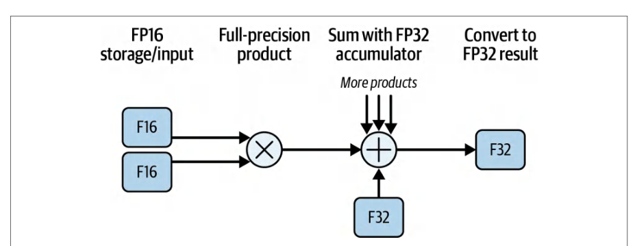
In PyTorch, these mixed-precision decisions are integrated into the compiler so you get optimal dtype selection (e.g., FP16/FP8 for compute, FP32 for accumulations) without requiring manual intervention. This is shown in Figure 9-7 as a mixed-precision matrix multiply-accumulate (MMA).在 PyTorch 中,这些混合精度决策已集成到编译器中,因此无需人工干预即可获得最优的 dtype 选择(例如计算用 FP16/FP8,累加用 FP32)。图 9-7 以混合精度矩阵乘累加(MMA)展示了这一点。
This automatic mixed-precision pipeline maximizes arithmetic intensity with minimal code changes. The fused Tensor Core kernels minimize round trips to HBM by staging and reusing data in shared memory (e.g., operands) and TMEM (e.g., accumulators).这种自动混合精度流水线以最少的代码改动最大化算术强度。融合后的张量核心内核通过在共享内存(例如操作数)和 TMEM(例如累加器)中暂存并复用数据,最大限度减少往返 HBM 的次数。
When using structured sparsity, described earlier, or extreme low-precision (FP8/ FP4), be sure to maintain a large enough batch size or tile granularity so that TMEM and Tensor Cores remain fully utilized. Small batches incur overhead, including format conversions, sparse index handling, irregular memory patterns, etc. This can reduce achieved speedups.使用前文所述的结构化稀疏性,或极低精度(FP8/FP4)时,务必保持足够大的批大小或 tile 粒度,使 TMEM 与张量核心保持充分利用。小批量会带来额外开销,包括格式转换、稀疏索引处理、不规则显存访问模式等。这会降低实际获得的加速比。
For example, when using FP8 or 2:4 sparsity, a batch size of 1 may see little benefit because the fixed overhead isn’t amortized. In contrast, a batch size of 128 or 256 will fully utilize the TMEM pipeline and produce near-peak throughput.例如,使用 FP8 或 2:4 稀疏性时,批大小为 1 可能几乎看不到收益,因为固定开销无法被摊薄。相比之下,批大小为 128 或 256 时能充分利用 TMEM 流水线,并产生接近峰值的吞吐量。
BF16/FP16、FP8 与 FP4 低精度
BF16/FP16, FP8, and FP4 Reduced Precision
BF16/FP16 (half-precision) has been supported for many GPU generations, but Tensor Cores on modern GPUs can often sustain greater than 90% of the BF16/FP16 peak throughput, around 4× the FP32 peak throughput. This is because at each cycle, the hardware issues many BF16/FP16 FMA operations in parallel.BF16/FP16(半精度)已在多代 GPU 上获得支持,而现代 GPU 上的张量核心通常能维持超过 90% 的 BF16/FP16 峰值吞吐量,约为 FP32 峰值吞吐量的 4 倍。这是因为在每个时钟周期内,硬件会并行发射大量 BF16/FP16 FMA 运算。
FP16 training uses a narrower 5-bit exponent than FP32, so very small gradient values can underflow to zero unless you apply loss scaling. Loss scaling preserves numerical stability during backpropagation. This scaling can either be static or dynamic.FP16 训练使用的指数位宽为 5 位,比 FP32 更窄,因此极小的梯度值会下溢为零,除非施加损失缩放。损失缩放可在反向传播过程中保持数值稳定性。这种缩放既可以是静态的,也可以是动态的。
In contrast, BF16 matches FP32’s 8-bit exponent range and natively avoids underflow. There, it rarely (if ever) requires loss scaling. This simplifies mixed-precision workflows and often improves training accuracy on modern GPUs.相比之下,BF16 与 FP32 一样具有 8 位指数范围,原生即可避免下溢。因此它很少(甚至几乎不需要)使用损失缩放。这简化了混合精度工作流,并且通常能提升现代 GPU 上的训练精度。
To push throughput even higher, you can use FP8. By reducing 16-bit weights by 50% down to 8 bits, you cut memory traffic in half—and double the number of weights loaded per HBM transaction. In practice, FP8 matmuls with FP32 or TF32 accumulation achieve 2–3× the BF16/FP16 TFLOPS—assuming that the model’s slight loss in accuracy due to quantization errors remains acceptable.若要进一步推高吞吐量,可以使用 FP8。将 16 位权重减少 50% 降至 8 位后,显存流量减半,并且每次 HBM 事务加载的权重数量翻倍。在实践中,采用 FP32 或 TF32 累加的 FP8 matmul 可达到 BF16/FP16 TFLOPS 的 2–3 倍——前提是模型因量化误差而出现的轻微精度损失仍可接受。
To address accuracy concerns at very low precision, the Transformer Engine supports FP8 as well as NVIDIA’s 4-bit NVFP4 format with micro-scaling. NVFP4 applies two-level scaling, combining per-microblock scaling and a higher-level scale so that models can retain accuracy while using 4-bit storage for weights. In addition, Blackwell B200’s NVFP4’s aggressive microscaling quantization provides 10 petaFLOPS (dense), while FP32 peak is about 80 teraFLOPS (dense). This is a speedup of approximately two orders of magnitude higher theoretical throughput per weight. And Blackwell’s B300 (Ultra) boasts 50% higher NVFP4 compute capacity than B200 at 15 petaFLOPS (dense).为解决极低精度下的精度问题,Transformer Engine 支持 FP8 以及 NVIDIA 带微缩放的 4 位 NVFP4 格式。NVFP4 采用两级缩放,将逐微块缩放与更高层级的缩放因子相结合,使模型在使用 4 位存储权重的同时仍能保持精度。此外,Blackwell B200 的 NVFP4 激进微缩放量化可提供 10 petaFLOPS(稠密),而 FP32 峰值约为 80 teraFLOPS(稠密)。这意味着每个权重的理论吞吐量提升了约两个数量级。而 Blackwell B300(Ultra)的 NVFP4 算力比 B200 高出 50%,达到 15 petaFLOPS(稠密)。
If your model tolerates the precision drop after calibration, NVFP4 kernels can deliver substantially higher throughput than FP32 on supported hardware, but accuracy must be validated per model.如果你的模型能够容忍校准后的精度下降,那么在受支持的硬件上,NVFP4 内核可以带来远高于 FP32 的吞吐量,但必须针对每个模型验证精度。
And since the precision is so low, the 256 KB TMEM per SM can hold large FP4 tiles (e.g., 256 × 256), which further increases on-chip reuse and improves performance. Note that all low-precision → accumulation conversions happen automatically. The kernel reads FP4 inputs from HBM, the Tensor Cores perform FP4 × FP4 multiplies, and the MMA API accumulates the results into BF16/FP16 or FP32 accumulators.由于精度如此之低,每个 SM 的 256 KB TMEM 可以容纳大型 FP4 tile(例如 256 × 256),这进一步提高了片上复用率并改善性能。请注意,所有低精度→累加的转换都会自动完成。内核从 HBM 读取 FP4 输入,张量核心执行 FP4 × FP4 乘法,MMA API 将结果累加到 BF16/FP16 或 FP32 累加器中。
Each drop in precision doubles or quadruples the number of operations per byte and therefore increases arithmetic intensity. When TMEM/TMA overlap memory and compute, these low-precision formats turn formerly memory-bound kernels into entirely compute-bound ones. This fully utilizes the multi-PFLOPS-per-GPU Tensor Core engines in modern GPUs.精度每降低一档,每字节的运算次数就会翻倍或增至四倍,从而提升算术强度。当 TMEM/TMA 将显存访问与计算重叠时,这些低精度格式会把原本受内存限制的内核转变为完全受计算限制的内核。这充分利用了现代 GPU 中每 GPU 数 PFLOPS 的张量核心引擎。
INT8 低精度与用于推理的 DP4A 指令
INT8 Reduced Precision and DP4A Instructions for Inference
LLM inference use cases can typically tolerate reduced-precision INT8 quantization supported by modern GPUs using DP4A (SIMD dot-product) instructions on regular CUDA cores and integer matrix-multiply/accumulate (MMA) instructions on Tensor Cores. At the instruction level, DP4A performs four INT8 multiply-accumulate (MAC) operations per instruction compared to one FP32 fused multiply-add (FMA) per instruction.LLM 推理用例通常可以容忍现代 GPU 所支持的降精度 INT8 量化,这类 GPU 在普通 CUDA 核心上使用 DP4A(SIMD 点积)指令,在张量核心上使用整数矩阵乘累加(MMA)指令。在指令层面,DP4A 每条指令执行四次 INT8 乘累加(MAC)运算,而每条指令只执行一次 FP32 融合乘加(FMA)。
Because weight traffic for INT8 is only one byte per element instead of four bytes for FP32, memory traffic for weights drops by 75%. INT8 inference workloads can significantly outperform FP32 due to higher peak INT8 Tensor Core throughput and reduced memory traffic. This is because each GPU can process approximately 4×由于 INT8 的权重传输每个元素仅占一个字节,而 FP32 需要四个字节,因此权重的内存传输量下降了 75%。得益于更高的 INT8 张量核心峰值吞吐量和更少的内存传输量,INT8 推理工作负载的性能可以显著优于 FP32。这是因为在使用 INT8 权重时,每块 GPU 每秒可从内存中处理大约 4×
more data per second from memory when using INT8 weights. This is made possible by TMEM and TMA keeping data and compute perfectly overlapped—and feeding the Tensor Cores as efficiently as possible.的数据量。这得益于 TMEM 和 TMA 使数据与计算完美重叠,并以尽可能高效的方式为张量核心供给数据。
深入解析 Transformer Engine 与 TMEM
Transformer Engine and TMEM in Depth
Modern NVIDIA GPUs include a Transformer Engine that combines Tensor Core hardware support for low-precision formats with a software runtime for scaling and casting. Kernels in cuBLASLt, cuDNN, CUTLASS, or OpenAI’s Triton perform cp.async instructions or TMA transfers into shared memory. The Tensor Core instructions then move operands between shared memory and TMEM implicitly.现代 NVIDIA GPU 包含 Transformer Engine,它将张量核心对低精度格式的硬件支持与用于缩放和类型转换的软件运行时结合在一起。cuBLASLt、cuDNN、CUTLASS 或 OpenAI 的 Triton 中的内核会执行 cp.async 指令或 TMA 传输,将数据送入共享内存。随后,张量核心指令会隐式地在共享内存与 TMEM 之间移动操作数。
Remember that TMEM is the 256 KB per-SM SRAM buffer that the Transformer Engine and Tensor Cores use to store results (instead of registers). In practice, you never explicitly allocate TMEM. It’s all handled by the hardware. For instance, when invoking Tensor Core’s MMA operations, the hardware handles all of the memory allocations and data transfers.请记住,TMEM 是每个 SM 256 KB 的 SRAM 缓冲区,Transformer Engine 和张量核心用它来存储结果(而不是使用寄存器)。在实践中,你从不需要显式分配 TMEM,这一切都由硬件处理。例如,在调用张量核心的 MMA 运算时,硬件会处理所有的显存分配和数据传输。
With the MMA instructions, each warp directly drives the Tensor Cores to perform high-throughput mixed-precision MMA operations. These operations manage fragment loads, register mappings, and mixed-precision MMA operations.借助 MMA 指令,每个线程束直接驱动张量核心执行高吞吐量的混合精度 MMA 运算。这些运算负责管理片段加载、寄存器映射以及混合精度 MMA 运算。
Any time you launch a Tensor-Core-based kernel or a GEMM library function (e.g., CUTLASS), the implementation manages operand movement through shared memory and TMEM automatically. This keeps the Tensor Cores full of tiles that are ready to be processed. (Note that the application code does not allocate TMEM directly.)每当你启动基于张量核心的内核或 GEMM 库函数(例如 CUTLASS)时,其实现都会自动管理操作数经由共享内存和 TMEM 的移动。这使张量核心始终充满待处理的瓦片(tile)。(请注意,应用代码不会直接分配 TMEM。)
The Transformer Engine workflow is straightforward. First, your kernel issues a MMA call or launches a CUTLASS GEMM. Next, the Transformer Engine’s firmware arranges for TMA (or cuda::memcpy_async) to copy weights and activations from HBM into shared memory (SMEM). Tensor Core instructions (e.g., tcgen05.mma) then move operands between SMEM and TMEM implicitly during the MMA pipeline. Ideally, the weights are in FP8 or FP4, and the activations are cast to FP8/FP4 when possible—otherwise, the activations can be left in FP16/FP32 format.Transformer Engine 的工作流程很直接。首先,你的内核发出 MMA 调用或启动 CUTLASS GEMM。接着,Transformer Engine 的固件安排 TMA(或 cuda::memcpy_async)将权重和激活值从 HBM 复制到共享内存(SMEM)。随后,张量核心指令(例如 tcgen05.mma)在 MMA 流水线执行期间隐式地在 SMEM 与 TMEM 之间移动操作数。理想情况下,权重采用 FP8 或 FP4 格式,激活值在可能时被转换为 FP8/FP4——否则,激活值可以保持 FP16/FP32 格式。
Tensor Core MMA operations execute at low precision, such as FP8 × FP8 with higher-precision accumulation or FP16 × FP16 with FP32 accumulation. Partial sums accumulate in TMEM with higher precision (e.g., BF16, FP16, FP32) and are kernel dependent. The accumulator state resides in TMEM. This state is accessed using tcgen05 load and store interfaces. The hardware manages these moves transparently.张量核心 MMA 运算以低精度执行,例如 FP8 × FP8 配合更高精度的累加,或 FP16 × FP16 配合 FP32 累加。部分和在 TMEM 中以更高精度(例如 BF16、FP16、FP32)累加,具体取决于内核。累加器状态驻留在 TMEM 中。该状态通过 tcgen05 加载和存储接口访问。硬件会透明地管理这些移动。
If you build a custom tile loop, you can overlap data movement with Tensor Core compute. You can do this using cuda::memcpy_async and the CUDA Pipeline API, as shown in the code here:如果你构建自定义的瓦片循环,就可以让数据移动与张量核心计算重叠。你可以使用 cuda::memcpy_async 和 CUDA Pipeline API 来实现,如下面的代码所示:
#include <cuda/pipeline>
#include <cooperative_groups.h>
namespace cg = cooperative_groups;
extern "C" __global__
void double_buffer_a(const float* __restrict__ globalA,
                     int tile_elems,
                     int numTiles) {
  __shared__ float tileA0[TILE][TILE];
  __shared__ float tileA1[TILE][TILE];
  auto block = cg::this_thread_block();
  constexpr auto scope = cuda::thread_scope_block;
  constexpr int stages = 2;
  __shared__ cuda::pipeline_shared_state<scope, stages> pstate;
  auto pipe = cuda::make_pipeline(block, &pstate);
  // 用分块 0 预热流水线
  pipe.producer_acquire();
  cuda::memcpy_async(block,
                     &tileA0[0][0],
                     globalA + 0 * tile_elems,
                     cuda::aligned_size_t<32>{tile_elems * sizeof(float)}
                     pipe);
  pipe.producer_commit();
  for (int t = 1; t < numTiles; ++t) {
    // 将下一个分块暂存到备用缓冲区
    pipe.producer_acquire();
    float* nxtA = (t & 1) ? &tileA1[0][0] : &tileA0[0][0];
    cuda::memcpy_async(block,
                       nxtA,
                       globalA + t * tile_elems,
                       cuda::aligned_size_t<32>{tile_elems * sizeof(float)}
                       pipe);
    pipe.producer_commit();
    // 使用此前暂存的分块
    pipe.consumer_wait();
    float* curA = ((t - 1) & 1) ? &tileA1[0][0] : &tileA0[0][0];
    pipe.consumer_release();
  }
  // 使用最后暂存的分块
#include <cuda/pipeline>
#include <cooperative_groups.h>
namespace cg = cooperative_groups;
extern "C" __global__
void double_buffer_a(const float* __restrict__ globalA,
                     int tile_elems,
                     int numTiles) {
  __shared__ float tileA0[TILE][TILE];
  __shared__ float tileA1[TILE][TILE];
  auto block = cg::this_thread_block();
  constexpr auto scope = cuda::thread_scope_block;
  constexpr int stages = 2;
  __shared__ cuda::pipeline_shared_state<scope, stages> pstate;
  auto pipe = cuda::make_pipeline(block, &pstate);
  // Prime pipeline with tile 0
  pipe.producer_acquire();
  cuda::memcpy_async(block,
                     &tileA0[0][0],
                     globalA + 0 * tile_elems,
                     cuda::aligned_size_t<32>{tile_elems * sizeof(float)}
                     pipe);
  pipe.producer_commit();
  for (int t = 1; t < numTiles; ++t) {
    // Stage next tile into the alternate buffer
    pipe.producer_acquire();
    float* nxtA = (t & 1) ? &tileA1[0][0] : &tileA0[0][0];
    cuda::memcpy_async(block,
                       nxtA,
                       globalA + t * tile_elems,
                       cuda::aligned_size_t<32>{tile_elems * sizeof(float)}
                       pipe);
    pipe.producer_commit();
    // Consume the previously staged tile
    pipe.consumer_wait();
    float* curA = ((t - 1) & 1) ? &tileA1[0][0] : &tileA0[0][0];
    pipe.consumer_release();
  }
  // Consume the final staged tile
  pipe.consumer_wait();
  float* lastA = ((numTiles - 1) & 1) ? &tileA1[0][0] : &tileA0[0][0];
  // 将 lastA 用于你的计算
  pipe.consumer_release();
}
  pipe.consumer_wait();
  float* lastA = ((numTiles - 1) & 1) ? &tileA1[0][0] : &tileA0[0][0];
  // Use lastA with your compute
  pipe.consumer_release();
}
Because TMEM is a dedicated on-chip buffer used by Tensor Core instructions, data is kept close to the compute units. While Tensor Cores process the current tile, cuda::memcpy_async streams the next tile from HBM into shared memory.由于 TMEM 是张量核心指令专用的片上缓冲区,数据被保持在靠近计算单元的位置。当张量核心处理当前分块时,cuda::memcpy_async 会将下一个分块从 HBM 流式传输到共享内存。
This overlap helps hide memory latency and can keep Tensor Cores busy when the pipeline is tuned. This collaboration between the Transformer Engine, TMEM, and TMA can substantially raise arithmetic intensity and approach speed-of-light efficiency in optimized cases.这种重叠有助于隐藏内存时延,并且在流水线调优得当时能让张量核心保持忙碌。Transformer Engine、TMEM 与 TMA 之间的这种协作可以显著提升算术强度,并在优化良好的情况下接近光速(speed-of-light)效率。
使用 CUTLASS 实现最优算术强度与张量核心性能
Using CUTLASS for Optimal Arithmetic Intensity and Tensor Core Performance
One of the easiest ways to leverage these optimizations yourself is to use NVIDIA’s CUTLASS library. With CUTLASS, you write a single templated call, and it will automatically apply many advanced optimizations.要亲自利用这些优化,最简单的方法之一是使用 NVIDIA 的 CUTLASS 库。借助 CUTLASS,你只需编写一个模板化调用,它就会自动应用许多高级优化。
Some optimizations that CUTLASS applies are shared-memory tiling, asynchronous memory transfers, and double buffering with the help of TMEM’s 256 KB per-SM buffer. This way, your Tensor Cores run at near-peak throughput without any manual kernel tuning.CUTLASS 应用的部分优化包括共享内存分块、异步内存传输,以及借助 TMEM 每 SM 256 KB 缓冲区实现的双缓冲。这样一来,无需任何手动内核调优,你的张量核心就能以接近峰值的吞吐量运行。
For example, suppose you want to compute a GEMM, C = A * B, with half-precision inputs and a half-precision output accumulating in FP16 or FP32 as appropriate. Instead of writing a hand-tuned MMA loop, you can simply include CUTLASS and instantiate a template, as shown in the following code:例如,假设你要计算一个 GEMM,C = A * B,输入为半精度,输出为半精度,并按需以 FP16 或 FP32 累加。无需编写手工调优的 MMA 循环,你只需包含 CUTLASS 并实例化一个模板,如下方代码所示:
#include <cutlass/numeric_types.h>
#include <cutlass/gemm/device/gemm.h>
using Gemm = cutlass::gemm::device::Gemm<
  cutlass::half_t,  // A(FP16)
  cutlass::layout::RowMajor,
  cutlass::half_t,  // B(FP16)
  cutlass::layout::ColumnMajor,
  cutlass::half_t,  // C / 输出(FP16)
  cutlass::layout::RowMajor,
  float, // 累加器(FP32 累加)
  cutlass::arch::OpClassTensorOp,
  cutlass::arch::Sm100 // 例如 Blackwell B200
>;
// ……(分配设备指针 A_d、B_d、C_d,
// 设置维度 M、N、K,以及步长 lda、ldb、ldc)……
Gemm gemm_op;
cutlass::Status status = gemm_op(
    { M, N, K },              // GEMM 形状
    float(1.0f)               // alpha
    A_d, lda,                 // A 指针 + 前导维度
    B_d, ldb,                 // B 指针 + 前导维度
    float(0.0f),              // beta
    C_d, ldc                  // C 指针 + 前导维度
);
#include <cutlass/numeric_types.h>
#include <cutlass/gemm/device/gemm.h>
using Gemm = cutlass::gemm::device::Gemm<
  cutlass::half_t,  // A (FP16)
  cutlass::layout::RowMajor,
  cutlass::half_t,  // B (FP16)
  cutlass::layout::ColumnMajor,
  cutlass::half_t,  // C / output (FP16)
  cutlass::layout::RowMajor,
  float, // accumulator (FP32 accumulate)
  cutlass::arch::OpClassTensorOp,
  cutlass::arch::Sm100 // e.g., Blackwell B200
>;
// ... (allocate device pointers A_d, B_d, C_d,
// set up dimensions M,N,K, and strides lda, ldb, ldc) ...
Gemm gemm_op;
cutlass::Status status = gemm_op(
    { M, N, K },              // GEMM shape
    float(1.0f)               // alpha
    A_d, lda,                 // A pointer + leading dimension
    B_d, ldb,                 // B pointer + leading dimension
    float(0.0f),              // beta
    C_d, ldc                  // C pointer + leading dimension
);
When you compile and run this code, CUTLASS does several key things automatically. First, CUTLASS selects tiles to balance register pressure, shared memory capacity, and Tensor Core utilization. On modern GPUs, TMEM exists alongside shared memory and L1. CUTLASS stages tiles in shared memory and uses Tensor Core instructions that interact with TMEM to store accumulator data. The tile shapes are chosen empirically and per-kernel. For instance, it may select tile sizes such as 128 × 128 or 256 × 128. These would fit into TMEM’s 256 KB per-SM buffer and would remain on-chip throughout the Tensor Core computation.当你编译并运行这段代码时,CUTLASS 会自动完成几项关键工作。首先,CUTLASS 会选择分块,以平衡寄存器压力、共享内存容量和张量核心利用率。在现代 GPU 上,TMEM 与共享内存和 L1 并存。CUTLASS 将分块暂存到共享内存,并使用与 TMEM 交互的张量核心指令来存储累加器数据。分块形状是依据经验、针对每个内核选定的。例如,它可能选择 128 × 128 或 256 × 128 这样的分块尺寸。这些分块能够放入 TMEM 每 SM 256 KB 的缓冲区,并在整个张量核心计算过程中始终保留在片上。
Depending on the precision, a 256 × 512 tile would max out the 256 KB per-SM TMEM budget since 256 × 512 elements × 2 bytes per element = 256 KiB. And 256 × 256 elements × 4 bytes per element = 256 KB. Larger tiles improve per-tile throughput but reduce the number of concurrent tiles per SM. This can lead to underutilization on smaller GEMMs. In contrast, very small tiles sacrifice arithmetic intensity for parallelism.取决于精度,256 × 512 的分块会耗尽每 SM 256 KB 的 TMEM 预算,因为 256 × 512 个元素 × 每元素 2 字节 = 256 KiB。而 256 × 256 个元素 × 每元素 4 字节 = 256 KB。更大的分块可提升单分块吞吐量,但会减少每个 SM 上并发分块的数量。这可能导致在较小的 GEMM 上出现利用率不足。相反,极小的分块会以牺牲算术强度来换取并行度。
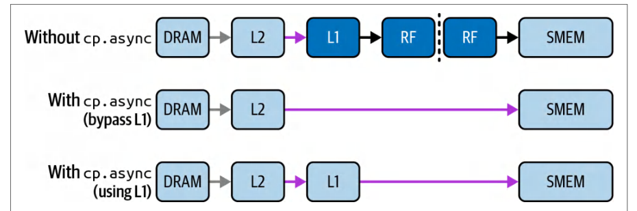
CUTLASS then emits asynchronous memory copies (cp.async or TMA) that stream each tile from DRAM into shared memory. The cp.async instruction stages data from global memory into shared memory without using per-thread registers (or optionally L1 cache), as shown in Figure 9-8. The caching behavior is controlled using cp.async modifiers or by using TMA for bulk tensor transfers.随后,CUTLASS 会发出异步内存复制(cp.async 或 TMA),将每个分块从 DRAM 流式传输到共享内存。cp.async 指令将数据从全局内存暂存到共享内存,而不使用每线程寄存器(也可选择不使用 L1 缓存),如图 9-8 所示。缓存行为通过 cp.async 修饰符控制,或通过使用 TMA 进行批量张量传输来控制。
CUTLASS stages tiles from global DRAM into SMEM using cp.async or TMA (cp.async.bulk.tensor). Tensor Core tcgen05.mma instructions then read operands from SMEM and accumulate the results implicitly into TMEM. This creates a software-managed staging area in shared memory, which is used for double-buffering. This way, while the Tensor Cores are processing the current tile, TMA is already fetching the next tile into shared memory.CUTLASS 使用 cp.async 或 TMA(cp.async.bulk.tensor)将分块从全局 DRAM 暂存到 SMEM。随后,张量核心的 tcgen05.mma 指令从 SMEM 读取操作数,并将结果隐式累加到 TMEM 中。这在共享内存中构建出一块由软件管理的暂存区,用于实现双缓冲。这样一来,当张量核心正在处理当前分块时,TMA 已经在把下一个分块取入共享内存。
Using the CUDA Pipeline API and warp-specialized compute stages (discussed in the next chapter), CUTLASS keeps all of the Tensor Core pipelines busy. It accumulates partial sums in the precision that you specify (for example, FP32 when inputs are FP16 or FP8) to ensure numerical fidelity—and then writes the results from TMEM out to shared or global memory in a coalesced fashion.借助 CUDA Pipeline API 与线程束专用化的计算阶段(将在下一章讨论),CUTLASS 让所有张量核心流水线保持忙碌。它按你指定的精度累加部分和(例如输入为 FP16 或 FP8 时使用 FP32),以确保数值保真度,然后以合并访问的方式将结果从 TMEM 写回共享内存或全局内存。
Because all of this complexity is hidden, CUTLASS gives you a drop-in, high-performance GEMM kernel that matches a hand-tuned MMA kernel—often within a few percent of overall Tensor Core utilization and performance compared to the hand-written version, as shown in Table 9-1.由于所有这些复杂性都被隐藏起来,CUTLASS 为你提供了一个可直接替换的高性能 GEMM 内核,其表现可与手工调优的 MMA 内核相媲美——如表 9-1 所示,与手写版本相比,整体张量核心利用率和性能通常只相差几个百分点。
| Metric指标 | Hand-tuned MMA kernel手工调优的 MMA 内核 | CUTLASS GEMMCUTLASS GEMM |
|---|---|---|
| Tensor Core utilization张量核心利用率 | 98%98% | 98%98% |
| Registers per thread每线程寄存器数 | ~52~52 | ~60 (slightly higher)~60(略高) |
| Shared memory per thread block (CTA)每线程块(CTA)共享内存 | ~2 KB~2 KB | ~4 KB~4 KB |
| Development effort开发工作量 | High高 | Low (simple template configuration)低(简单的模板配置) |
Here, both use FP16 inputs with FP32 accumulation. And both aim to maximize Tensor Core utilization. As the table shows, CUTLASS matches or exceeds hand-tuned MMA performance within about 2%. And although CUTLASS used a few more registers and doubled the shared memory in this case, it stayed well within the hardware limits. The slight increases do not impact occupancy.这里,两者都使用 FP16 输入与 FP32 累加。并且两者都旨在最大化张量核心利用率。如表所示,CUTLASS 在约 2% 的范围内匹配或超越手工调优的 MMA 性能。尽管在此案例中 CUTLASS 多用了几个寄存器,并将共享内存翻倍,但它仍远在硬件限制之内。这些轻微的增量并不影响占用率。
It requires only a few lines of template code instead of weeks of low-level tuning. In addition, CUTLASS templates already support FP4, FP8, FP16, and TF32 operand types. And they can fuse common postprocessing operations like bias-add and activation into the same kernel.它只需要几行模板代码,而不是数周的低层调优。此外,CUTLASS 模板已经支持 FP4、FP8、FP16 和 TF32 操作数类型。并且它们可以把偏置相加和激活等常见后处理操作融合进同一个内核。
This is in contrast to writing a custom MMA kernel, which requires manually selecting tile sizes, writing asynchronous copy loops, managing double buffers, implementing warp specialization pipelines, and thread block cluster tiles. All of this is done for you automatically with CUTLASS.这与编写自定义 MMA 内核形成对比:后者需要手动选择分块尺寸、编写异步拷贝循环、管理双缓冲、实现线程束专用化流水线以及线程块集群分块。而所有这些在 CUTLASS 中都会自动为你完成。
Optimized libraries such as cuBLAS are built on CUTLASS. And high-level libraries like PyTorch call these optimized libraries for many kernels. In our earlier fused-attention example, we showed that TorchInductor dispatched a CUTLASScuBLAS 等优化库构建在 CUTLASS 之上。而像 PyTorch 这样的高层库在许多内核中都会调用这些优化库。在我们先前的融合注意力示例中,我们展示了 TorchInductor 调度了一个 CUTLASS
fused-attention kernel that used exactly the same double-buffered TMEM pipeline. This results in 98% Tensor Core utilization and near-zero memory stalls.融合注意力内核,它使用了完全相同的双缓冲 TMEM 流水线。这带来了 98% 的张量核心利用率和接近零的内存停顿。
There may still be scenarios in which you need to write a manual MMA kernel—for instance, when you need a highly specialized data layout or a unique fusion pattern that CUTLASS does not yet support.仍可能存在需要你编写手动 MMA 内核的场景——例如,当你需要高度专用的数据布局,或 CUTLASS 尚不支持的独特融合模式时。
In these cases, you would need to implement this complexity yourself. You would first need to choose a tile size that fits within TMEM (e.g., 128 × 128 FP16), then use <cuda/pipeline> to perform asynchronous memory copy (cp.async) instructions for each tile.在这些情况下,你就需要自己实现这些复杂度。你首先需要选择一个能放进 TMEM 的分块尺寸(例如 128 × 128 FP16),然后使用 <cuda/pipeline> 为每个分块执行异步显存拷贝(cp.async)指令。
You would then need to implement warp-specialized MMA loops and double-buffer TMEM to hide DRAM latency. Last, you would interleave any custom postprocessing steps like softmax and elementwise nonlinearities—all within the same loop, if possible.随后你需要实现线程束专用化的 MMA 循环,并对 TMEM 做双缓冲,以隐藏 DRAM 时延。最后,你还要把 softmax、逐元素非线性等自定义后处理步骤交织进来——如果可能,全部放在同一个循环内。
However, for almost every standard GEMM or fused-attention use case, CUTLASS and the libraries built on it are the recommended approach.不过,对于几乎所有标准 GEMM 或融合注意力用例,CUTLASS 以及基于它构建的库都是推荐方案。
Its template-based design, GPU-specific tuning, and built-in support for TMEM and TMA pipelines typically achieve high Tensor Core utilization on supported shapes. This allows you to achieve 96%–98% Tensor Core utilization, in some cases, with minimal developer effort.其基于模板的设计、针对特定 GPU 的调优,以及对 TMEM 和 TMA 流水线的内置支持,通常能在受支持的形状上实现高张量核心利用率。在某些情况下,这让你只需极少的开发投入就能达到 96%–98% 的张量核心利用率。
By depending on CUTLASS’s automatic optimizations, you can spend your time on model architecture, numeric precision strategies, and end-to-end performance. CUT-LASS gives you the confidence that your low-level tensor operations will run at near-peak arithmetic intensity optimized for your specific GPU hardware.依靠 CUTLASS 的自动优化,你可以把时间花在模型架构、数值精度策略和端到端性能上。CUTLASS 让你有信心:底层张量运算将以接近峰值的算术强度运行,并针对你的特定 GPU 硬件进行优化。
用于微优化的内联 PTX 与 SASS 调优
Inline PTX and SASS Tuning for Microoptimizations
For those willing to venture beyond C++ and into low-level microoptimizations, CUDA allows inline Parallel Thread Execution (PTX) code and SASS (NVIDIA’s assembly language) to bring out the last bits of performance that may be left on the table.对于愿意走出 C++、深入底层微优化的人,CUDA 允许内联并行线程执行(Parallel Thread Execution,PTX)代码和 SASS(NVIDIA 的汇编语言),以榨出可能尚未被利用的最后一点性能。
This is truly advanced territory, as the CUDA compiler is already quite good at optimization. But in some extreme cases, you can hand-schedule assembly instructions— or use special-purpose instructions—to gain a small percentage of performance gain in very specific situations.这确实属于高级领域,因为 CUDA 编译器在优化方面已经相当出色。但在某些极端情况下,你可以手工调度汇编指令——或使用专用指令——在非常特定的场景中获得几个百分点的性能提升。
With PTX and Streaming Assembler (SASS), you can also enable features not yet exposed in the higher-level CUDA language. Modern GPUs don’t typically introduce radical new assembly instructions, but they do offer opportunities for custom tuning. For instance, you can tweak the GPU caching strategy, modify the coordination of CPU-GPU unified memory access, and implement other fine-grained microoptimizations.借助 PTX 和流式汇编器(Streaming Assembler,SASS),你还可以启用高层 CUDA 语言尚未暴露的特性。现代 GPU 通常不会引入激进的新汇编指令,但确实提供了自定义调优的机会。例如,你可以调整 GPU 缓存策略、修改 CPU-GPU 统一内存访问的协调方式,以及实现其他细粒度微优化。
As an example, consider a piece of code in which you know that a specific instruction sequence would be optimal, but the compiler isn’t generating the specific sequence. Common scenarios include using a GPU instruction that has no direct CUDA intrinsic, applying memory load modifiers (cache hints) on specific accesses, inserting memory fences or barriers at precise points, or manually reordering instructions to avoid pipeline stalls.举例来说,假设有一段代码,你知道某个特定的指令序列是最优的,但编译器并没有生成该序列。常见场景包括:使用没有直接 CUDA 内建函数(intrinsic)的 GPU 指令、对特定访问施加内存加载修饰符(缓存提示)、在精确的位置插入内存栅栏或屏障,或手工重排指令以避免流水线停顿。
Another use is to read special registers or states such as SM ID, warp lane ID, etc., which might not have a high-level API. Inline PTX lets you embed assembly right in your CUDA C++ code using asm() statements. You can mix C++ and PTX by specifying inputs and outputs to the assembly code. The compiler will then incorporate your PTX instructions into the final SASS.另一个用途是读取特殊寄存器或状态,例如 SM ID、线程束 lane ID 等,这些可能没有高层 API。内联 PTX 让你可以使用 asm() 语句把汇编直接嵌入 CUDA C++ 代码。通过为汇编代码指定输入和输出,你可以混用 C++ 与 PTX。随后编译器会把你的 PTX 指令并入最终的 SASS。
Let’s look at a simple example that uses an inline PTX directive to prefetch a global memory address into L2 cache. Here, we are using kernel-side prefetching using the PTX instruction cp.async.bulk.prefetch.global:我们来看一个简单示例,它使用内联 PTX 指令把全局内存地址预取到 L2 缓存。这里我们使用 PTX 指令 cp.async.bulk.prefetch.global 进行内核侧预取:
__global__ void PrefetchExample(const float *in, float *out) {
    // ……假设 idx 是当前线程的数据索引
    int idx = blockIdx.x * blockDim.x + threadIdx.x;
    // 手动将 in[] 的下一个缓存行(128B)预取到 L2:
    // 从全局内存预取 128B 到 L2。
    // 地址必须 16B 对齐
    // 且大小为 16B 的整数倍。
    asm volatile("cp.async.bulk.prefetch.L2.global [%0], %1;"
                 :: "l"(in + idx + 32), "n"(128));
    float x = in[idx];
    // (在使用 in[idx+32] 之前先做一些工作,为预取留出时间)
    out[idx] = x;
}
__global__ void PrefetchExample(const float *in, float *out) {
    // ... assume idx is our thread’s data index
    int idx = blockIdx.x * blockDim.x + threadIdx.x;
    // Manually prefetch the next cache line (128B) of in[] into L2:
    // Prefetch 128B from global to L2.
    // Address must be 16B-aligned
    // and size is a 16B multiple.
    asm volatile("cp.async.bulk.prefetch.L2.global [%0], %1;"
                 :: "l"(in + idx + 32), "n"(128));
    float x = in[idx];
    // (do some work here before using in[idx+32] to give time for prefetch)
    out[idx] = x;
}
In this snippet, the inline PTX cp.async.bulk.prefetch.L2.global [%0] uses the address operand we provide (in + idx + 32 bytes, i.e., 32 floats ahead) and issues a prefetch to L2. We mark it volatile to ensure the compiler doesn’t optimize it away.在这段代码中,内联 PTX cp.async.bulk.prefetch.L2.global [%0] 使用我们提供的地址操作数(in + idx + 32 字节,即向前 32 个 float),并向 L2 发起预取。我们将其标记为 volatile,以确保编译器不会把它优化掉。
These PTX instructions will be injected into the machine code. Using inline assembly like this will give us very fine-grained control. For instance, we could prefetch to L2 or L1 (by using .L1) or choose the distance (32 floats ahead, in this case).这些 PTX 指令会被注入到机器码中。像这样使用内联汇编可以让我们获得非常细粒度的控制。例如,我们可以预取到 L2 或 L1(通过使用 .L1),也可以选择预取距离(本例中为向前 32 个 float)。
It’s essentially what __prefetch_async likely compiles down to. More generally, we can use inline PTX to control the caching behavior of normal loads. For example, we might write asm("ld.global.cg.f32 %0, [%1];" : "=f"(val) : "l"(ptr)) to load a float with the .cg (“cache global”) modifier.这本质上很可能就是 __prefetch_async 编译后生成的代码。更一般地说,我们可以用内联 PTX 控制普通加载的缓存行为。例如,我们可以写 asm("ld.global.cg.f32 %0, [%1];" : "=f"(val) : "l"(ptr)),用 .cg(“cache global”,缓存全局)修饰符加载一个 float。
On some architectures, this means we want to cache the data in L2 but bypass the L1 cache. If we knew a certain access was thrashing L1 and we preferred to use only L2, this could help. Normally, the compiler’s choice might default to caching in L1 (.ca), but we can use PTX to override the compiler’s decision.在某些架构上,这意味着我们希望把数据缓存在 L2 中而绕过 L1 缓存。如果我们知道某个访问正在反复冲刷 L1,而我们更希望只使用 L2,这就会有帮助。通常,编译器的选择可能默认缓存在 L1(.ca),但我们可以用 PTX 覆盖编译器的决定。
Another area in which inline PTX is helpful is instruction scheduling. By default, the compiler will issue instructions in the order that it deems optimal. But you might spot a case in which you want to intermix operations more effectively.内联 PTX 另一个有用的领域是指令调度。默认情况下,编译器会按它认为最优的顺序发射指令。但你可能会发现某种情况,你希望更有效地交错混合各个操作。
For instance, say you have two independent memory loads and then two uses of those results. The compiler might issue load1, then use1, then load2, then use2. But maybe the better instruction schedule is to perform load1 and load2 (back-to-back) and then use both results. This could overlap the memory latencies.例如,假设你有两个独立的内存加载,然后分别使用这两个结果。编译器可能会发射 load1、use1、load2、use2。但也许更好的指令调度是先执行 load1 和 load2(背靠背),然后再使用两个结果。这样可以重叠内存时延。
By writing inline PTX for the loads, you can enforce them early, then do the computations. This is a form of manually increasing ILP, discussed earlier. In practice, the compiler will already do a good job here since modern compilers try to fill load latency with other independent instructions. But inline PTX and SASS assembly can give you certainty.通过为这些加载编写内联 PTX,你可以强制它们提前执行,然后再做计算。这是前面讨论过的一种手动提高 ILP 的方式。在实践中,编译器在这里已经做得很好,因为现代编译器会尝试用其他独立指令填补加载时延。但内联 PTX 和 SASS 汇编可以给你确定性。
On modern CPU-GPU superchips that share CPU and GPU memory, such fine-grained control might be useful if you’re managing a workload in which the GPU polls a memory location updated by the CPU. Here, you could use appropriate memory fences such as membar.sys or __threadfence_system() together with the desired cache operators on loads and stores to ensure coherence at the intended scope. This is something that high-level CUDA might not expose directly.在共享 CPU 和 GPU 显存的现代 CPU-GPU 超级芯片上,如果你管理的负载中 GPU 会轮询由 CPU 更新的显存位置,这种细粒度控制可能很有用。此时,你可以使用适当的显存栅栏,例如 membar.sys 或 __threadfence_system(),配合加载和存储上所需的缓存操作符,以确保在预期作用域内的一致性。这是高层 CUDA 可能不会直接暴露的能力。
You can also use inline PTX to leverage special registers. For instance, although there’s no C++ intrinsic for SM ID (the SM that a thread block is running on), you can do asm("mov.u32 %0, %smid;" : "=r"(smid)) to get the SM ID. This flexibility is useful for debugging and work partitioning.你也可以用内联 PTX 来利用特殊寄存器。例如,尽管没有用于 SM ID(线程块正在其上运行的 SM)的 C++ 内建函数,你可以用 asm("mov.u32 %0, %smid;" : "=r"(smid)) 获取 SM ID。这种灵活性对调试和工作划分很有用。
Some developers have used %smid in persistent kernels to have only one block per SM do certain work, for instance. This effectively performs manual SM partitioning, which is beyond what the CUDA C++ API offers.例如,一些开发者在持久化内核中使用 %smid,让每个 SM 上只有一个线程块执行特定工作。这实际上执行了手动 SM 划分,超出了 CUDA C++ API 所提供的能力。
If your code is already well optimized at the algorithmic level, gains from inline PTX/ SASS tend to be just incremental and on the order of a few percent in most cases. For instance, in a memory-bound kernel you can carefully unroll and schedule instructions to reduce load-to-use latency bubbles and see maybe a 5%–10% speedup by using two independent load streams with PTX. In this case, the compiler may be more conservative.如果你的代码在算法层面已经充分优化,那么来自内联 PTX/SASS 的收益往往只是增量式的,在大多数情况下约为几个百分点。例如,在显存受限的内核中,你可以仔细地展开和调度指令,以减少从加载到使用的时延气泡,并通过用 PTX 使用两个独立的加载流获得大约 5%–10% 的加速。在这种情况下,编译器可能更为保守。
In a compute-bound scenario, you might use inline assembly to use a faster math instruction instead of a more precise instruction. CUDA provides fast math intrinsics for this, including __sinf().在计算受限的场景中,你可能会使用内联汇编来改用更快的数学指令,而不是更精确的指令。CUDA 为此提供了快速数学内建函数(fast math intrinsics),包括 __sinf()。
Before the C++ intrinsics were available, developers writing matrix multiply kernels would sometimes embed PTX instructions to use Tensor Cores. Today, we have higher-level intrinsics for this purpose. But, in short, assembly lets you tap hardware features as soon as you know about them—without waiting for CUDA to support them.在 C++ 内建函数可用之前,编写矩阵乘法内核的开发者有时会嵌入 PTX 指令来使用张量核心。如今,我们已有为此目的提供的更高层内建函数。但简而言之,汇编让你一旦了解到某项硬件特性就能立即加以利用——无需等待 CUDA 对其提供支持。
| Version版本 | Warp stall (memory)线程束停顿(内存) | Issue IPC发射 IPC | Kernel time内核时间 | Speedup加速比 |
|---|---|---|---|---|
| Optimized C++ (compiler schedule)优化后的 C++(编译器调度) | 35% of cycles占周期的 35% | 1.51.5 | 1.07 ms1.07 ms | 1.0× base1.0× 基准 |
| Hand-tuned PTX (manual scheduling and hints)手工调优的 PTX(手动调度与提示) | 20% of cycles占周期的 20% | 1.61.6 | 1.00 ms1.00 ms | 1.07×1.07× |
Nsight Compute can help inform assembly tuning. By inspecting the “SASS throughput” metrics and the “Warp Stall Reasons,” you might identify a lot of stalls due to memory dependencies. You could attempt to reorder the loads as mentioned earlier.Nsight Compute 可以为汇编调优提供依据。通过查看“SASS throughput”指标和“Warp Stall Reasons”,你可能会发现大量由内存依赖导致的停顿。此时可以尝试像前面提到的那样重排加载顺序。
After your change, you’d hope to see less “Stall Memory Dependency”—and perhaps higher instruction issue rate for more instructions executed per cycle. Note that assembly tweaking is labor-intensive—and can reduce code portability.修改之后,你希望看到“Stall Memory Dependency”减少,并且指令发射率提高,从而每个周期执行更多指令。请注意,汇编层面的调整是劳动密集型工作,而且会降低代码可移植性。
It’s usually only worth it for very hot inner loops in which you’ve exhausted higher-level optimizations. Also, any change in GPU generation might require retuning and verifying that your assumptions still hold, including memory latencies, cache behavior, etc.通常只有在已经用尽高层优化手段、且内层循环极其热点时,这项工作才值得做。此外,GPU 代际的任何变化都可能需要重新调优,并验证你的假设(包括内存时延、缓存行为等)是否仍然成立。
To illustrate the potential microoptimizations, consider a scenario in which a kernel was already quite optimized but had one remaining bottleneck: a tight loop doing integer index calculations and memory loads.为了说明潜在的微优化,考虑这样一个场景:某个内核已经相当优化,但仍存在一个瓶颈——一个执行整数索引计算和内存加载的紧凑循环。
You can use inline PTX to compute the byte address in one instruction with mad.wide.u32 (base + index * stride). Next, issue the load as ld.global.cg to bypass L1 for this streaming access pattern. The result is that the loop uses fewer instructions and avoids L1 evictions. In this case, we squeeze about a 7% speedup in that kernel from 1.07 ms down to 1.0 ms. Table 9-2 summarizes a hypothetical before-and-after for optimized CUDA C++ versus hand-written PTX with manual scheduling and cache hints.你可以使用内联 PTX,通过一条 mad.wide.u32 (base + index * stride) 指令计算出字节地址。接着,针对这种流式访问模式,用 ld.global.cg 发起加载以绕过 L1。结果是该循环使用的指令更少,并避免了 L1 逐出。在这个例子中,我们为该内核争取到约 7% 的加速,从 1.07 ms 降到 1.0 ms。表 9-2 汇总了一个假设性的前后对比:优化后的 CUDA C++ 与手工编写、带手动调度和缓存提示的 PTX。
Here we see that after tuning, our kernel’s memory stalls decreased by overlapping loads, and cache hints reduced some latency. Additionally, we increased ILP and the instructions per cycle (IPC). This gave a 7% net improvement in overall kernel execution time.可以看到,调优之后,通过重叠加载减少了内核的内存停顿,缓存提示也降低了一部分时延。此外,我们提高了 ILP 和每周期指令数(IPC)。这使内核整体执行时间净改善 7%。
These numbers are in line with what to expect from manual assembly on an already-optimized kernel. In some cases, the gains might be larger if the compiler made a poor choice, for instance—and you can implement the fix. Otherwise, the gain is essentially zero if the compiler already chose the optimal implementation. It’s also possible to hurt performance with incorrect assembly ordering, so one must experiment and profile each change.这些数字与在已优化的内核上手工编写汇编所能预期的效果相符。在某些情况下,例如编译器做出了糟糕的选择而你能够实现修正,收益可能更大。反之,如果编译器已经选择了最优实现,收益基本为零。错误的汇编顺序还可能损害性能,因此必须对每一处修改进行实验和性能剖析。
Inline PTX and SASS assembly can be viewed as the last resort optimization tool. It provides ultimate control at the cost of complexity. It’s recommended to use this last resource when you need a hardware feature or instruction that isn’t accessible in CUDA C++—or when you have pinpointed a small piece of code where the compiler’s scheduling can be improved upon. Examples include custom memory access patterns (cache hints, prefetches), fine-grained synchronization or fences, and utilizing new instructions before they are officially supported.内联 PTX 和 SASS 汇编可以视为最后手段的优化工具。它以复杂性为代价提供终极的控制力。建议仅在以下情况动用这一最后资源:你需要某个 CUDA C++ 无法访问的硬件特性或指令,或者你已经精确定位到一小段代码,其编译器调度仍有改进空间。示例包括自定义显存访问模式(缓存提示、预取)、细粒度同步或 fence,以及在官方支持之前使用新指令。
When applying inline assembly, it’s especially important to verify the impact with profiling. You want to see reductions in stall reasons or instruction count as intended. Also, you should keep such code isolated and well-documented. It will likely need updates for new GPU architectures—especially if you use SASS assembly, which is not always forward-compatible.在应用内联汇编时,尤其重要的是通过性能剖析验证其影响。你希望看到停顿原因或指令数按预期减少。此外,应让这类代码保持隔离并有充分的文档记录。它很可能需要针对新的 GPU 架构进行更新,尤其是当你使用 SASS 汇编时,因为 SASS 并不总是向前兼容。
Inline PTX/SASS tuning is for expert-level tweaking to shave off extra latency or enforce a specific scheduling. It can produce modest speedups and enable certain custom behaviors, but it should come after exhausting all other high-level optimizations. For instance, you may want to handcraft the assembly for critical loops that run millions of times. At the very least, it’s an effective way to learn exactly how the hardware executes your code.内联 PTX/SASS 调优属于专家级的微调,用于削减额外时延或强制实施特定的调度。它可以带来适度的加速并实现某些自定义行为,但应当在用尽所有其他高层优化之后再考虑。例如,对于要执行数百万次的关键循环,你可能想手工编写其汇编。至少,它是精确了解硬件如何执行你的代码的有效途径。
In short, use inline PTX/SASS sparingly and profile diligently. The gains are real but usually incremental. The maintenance cost is much higher. For most use cases, relying on CUDA’s built-in optimizations—or highly tuned libraries like CUB and Thrust—is likely good enough. But it’s good to know that, if needed, you can drop to assembly and gain full control over the GPU.简而言之,谨慎使用内联 PTX/SASS,并勤于做性能剖析。收益是真实的,但通常是渐进式的;维护成本却高得多。对于大多数用例,依赖 CUDA 的内置优化——或 CUB、Thrust 等经过高度调优的库——很可能已经足够。但了解一下也好:如有需要,你可以下沉到汇编层面,获得对 GPU 的完全控制。
DeepSeek 使用内联 PTX 优化显存分配
DeepSeek’s Use of Inline PTX for Memory Allocation Optimization
A well-known example of custom PTX is from DeepSeek’s DeepEP expert parallelism library. This library used a bespoke PTX instruction, ld.global.nc.l1::no_allo cate.l2::256b, to optimize global memory access by bypassing L1 cache allocations, preserving critical data, and leveraging 256-byte L2 cache chunks. This is ideal for streaming large datasets directly into the L2 cache without disrupting frequent-access memory operations in the L1 cache.自定义 PTX 的一个著名例子来自 DeepSeek 的 DeepEP 专家并行库。该库使用了一条定制的 PTX 指令 ld.global.nc.l1::no_allo cate.l2::256b,通过绕过 L1 缓存分配、保留关键数据并利用 256 字节的 L2 缓存块来优化全局内存访问。这对于将大型数据集直接流式载入 L2 缓存、同时不干扰 L1 缓存中频繁访问的内存操作而言是理想之选。
This instruction is not part of NVIDIA’s official PTX ISA specification but was discovered “out-of-doc” by DeepSeek engineers to fine-tune cache behavior on their US-export-constrained H800 variant of the Hopper GPU.该指令并不属于 NVIDIA 官方 PTX ISA 规范,而是 DeepSeek 工程师“在文档之外”发现的,用于在其受美国出口限制的 Hopper GPU 变体 H800 上微调缓存行为。
Let’s break down the ld.global.nc.l1::no_allocate.l2::256b PTX instruction. The ld.global.nc prefix issues a noncoherent (nc) global memory load (ld.global), while the modifiers l1::no_allocate and l2::256b instruct the hardware to avoid allocating the data in the L1 cache (l1::no_allocate). Instead, it fetches 256 bytes at a time into L2 (l2::256b).让我们拆解 ld.global.nc.l1::no_allocate.l2::256b 这条 PTX 指令。ld.global.nc 前缀发起一次非一致性(nc)全局内存加载(ld.global),而修饰符 l1::no_allocate 和 l2::256b 指示硬件避免将数据分配到 L1 缓存(l1::no_allocate),而是每次取 256 字节到 L2(l2::256b)。
By bypassing L1, loads can stream large blocks of data directly into L2 without evict-ing frequently used L1-resident data. This is critical when you have hot working sets that need to stay in L1 for low-latency memory access.通过绕过 L1,加载可以将大块数据直接流式送入 L2,而不会逐出 L1 中常驻的频繁使用数据。当你拥有需要留在 L1 中以获得低时延显存访问的热点工作集时,这一点至关重要。
In practice, streaming workloads such as expert-parallel all-to-all communication kernels benefit from this approach because they often read large contiguous buffers exactly once per dispatch. If these loads went through L1, they could evict earlier cache lines that are still actively in use by the SMs.在实践中,诸如专家并行 all-to-all 通信内核之类的流式工作负载会受益于这种方法,因为它们通常每次分发只读取一次大型连续缓冲区。如果这些加载经过 L1,就可能逐出 SM 仍在活跃使用的较早缓存行。
By fetching in 256-byte aligned chunks directly into L2, the instruction reduces unnecessary L1 traffic. This helps maintain high throughput for both memory-bound communication and compute operations.通过以 256 字节对齐的块直接取入 L2,该指令减少了不必要的 L1 流量。这有助于为显存受限的通信操作和计算操作同时保持高吞吐量。
However, using PTX in this way carries some risks because ld.global.nc.l1::no_allo cate.l2::256b is not guaranteed to remain stable across GPU generations. As such, code that relies on it may break or produce incorrect results on future architectures.然而,以这种方式使用 PTX 存在一定风险,因为 ld.global.nc.l1::no_allo cate.l2::256b 并不保证在跨 GPU 代际时保持稳定。因此,依赖它的代码在未来的架构上可能失效或产生错误结果。
DeepSeek’s DeepEP setup even includes a build-time flag, DISABLE_AGGRES SIVE_PTX_INSTRS=1, to disable these aggressive instructions if compatibility issues arise. While DeepEP’s bespoke PTX hack can produce significant speedup, inline PTX/SASS should be used with caution and tested thoroughly whenever updating to a new GPU architecture.DeepSeek 的 DeepEP 配置甚至包含一个构建期标志 DISABLE_AGGRES SIVE_PTX_INSTRS=1,用于在出现兼容性问题时禁用这些激进指令。尽管 DeepEP 的定制 PTX 技巧能带来显著加速,但内联 PTX/SASS 应谨慎使用,并在升级到新的 GPU 架构时进行充分测试。
关键要点
Key Takeaways
You saw how to uncover and eliminate GPU kernel bottlenecks by moving work from slow global memory into faster on-chip resources and compute units. By following a cycle of profiling, diagnosing, optimizing, and reprofiling, you can transform kernels from underutilized or memory-bound into compute-saturated, high-throughput routines. These techniques will help utilize the full power of your GPUs:你已经了解了如何通过将工作从缓慢的全局内存迁移到更快的片上资源和计算单元,来发现并消除 GPU 内核瓶颈。遵循性能剖析、诊断、优化、再剖析的循环,你可以将内核从利用率不足或显存受限的状态转变为计算饱和的高吞吐量例程。这些技术将帮助你充分利用 GPU 的全部能力:
- Increase arithmetic intensity with tiling and fusion通过分块(tiling)与融合(fusion)提升算术强度
- To elevate FLOPS per byte transferred, stage data into shared memory and registers using multilevel tiling. Load a 32 × 32 submatrix into SMEM, for instance, so that each element is reused across many FMAs. Combine consecutive kernels by fusing elementwise operations so intermediate results stay on-chip. Utilize software prefetching through asynchronous memory loading with the CUDA Pipeline API’s
cuda::memcpy_asyncto overlap data movement with computation. This will hide DRAM latencies.为了提升每字节传输的 FLOPS,使用多级分块将数据暂存到共享内存和寄存器中。例如,将一个 32 × 32 的子矩阵加载到 SMEM,使每个元素在多次 FMA 中被复用。通过融合逐元素操作来合并连续的内核,使中间结果保留在片上。利用 CUDA Pipeline API 的cuda::memcpy_async进行异步内存加载以实现软件预取,从而将数据搬运与计算重叠。这将隐藏 DRAM 时延。
- Leverage mixed precision, Tensor Cores, and Transformer Engine利用混合精度、张量核心与 Transformer Engine
- Dropping from FP32 to TF32/BF16/FP16/FP8/FP4 cuts weight traffic by 2× to 8×. This boosts arithmetic intensity accordingly. In PyTorch, you can use
torch.set_float32_matmul_precision('high')andtorch.cuda.ampto enable mixed precision. On modern GPUs, the TMEM and TMA engines stream tiles to Tensor Cores. Modern GPUs also provide a Transformer Engine to utilize these lower precisions specifically for AI workloads. This can further increase throughput.从 FP32 降到 TF32/BF16/FP16/FP8/FP4,可将权重传输量削减 2× 到 8×,算术强度也随之提升。在 PyTorch 中,可以使用torch.set_float32_matmul_precision('high')和torch.cuda.amp启用混合精度。在现代 GPU 上,TMEM 与 TMA 引擎负责将数据块流式送入张量核心。现代 GPU 还提供 Transformer Engine,专门针对 AI 工作负载利用这些更低精度,从而进一步提升吞吐量。
- Utilize CUTLASS for high-performance GEMM and fused kernels利用 CUTLASS 实现高性能 GEMM 与融合内核
- Rather than hand-coding MMA loops, instantiate CUTLASS GEMM templates to automatically manage double buffering, TMEM staging, and Tensor Core pipelines. This will produce a kernel that performs within a few percent of a hand-tuned kernel. High-level frameworks like cuBLAS and TorchInductor already rely on CUTLASS. Customizations are needed only when you require nonstandard layouts or unique fusion patterns.与其手工编写 MMA 循环,不如实例化 CUTLASS GEMM 模板,由它自动管理双缓冲、TMEM 暂存与张量核心流水线。这样得到的内核,性能与手工调优内核相差仅几个百分点。cuBLAS 和 TorchInductor 等高层框架已经依赖 CUTLASS。只有当你需要非标准布局或独特的融合模式时,才需要做定制。
- PyTorch-specific best practicesPyTorch 专属最佳实践
- Favor built-in tensor operations such as
torch.matmul, fused attention, and nested tensors since PyTorch typically inherits Tensor Core and other hardware optimizations from CUDA over time. And if you write custom kernel extensions for PyTorch, carry over the same strategies: minimize register usage, align data for coalesced memory loads, and target Tensor Cores. This makes sure your kernels are at parity with native kernels.优先使用torch.matmul、融合注意力、嵌套张量等内置张量运算,因为 PyTorch 通常会随时间推移从 CUDA 继承张量核心等硬件优化。如果你为 PyTorch 编写自定义内核扩展,也要沿用同样的策略:最小化寄存器用量、对齐数据以实现合并显存访问、面向张量核心编程。这样才能确保你的内核与原生内核性能相当。
By following the systematic workflow of profiling, diagnosing, and applying targeted optimizations, from occupancy tuning and warp-level refinements to ILP and high arithmetic intensity with tiling, fusion, and Tensor Cores, you can transform a memory-bound GPU kernel into a compute-bound one. This can provide large speedups, and in strongly memory bound workloads, sometimes order-of-magnitude gains.遵循性能剖析、诊断、施加针对性优化的系统化流程——从占用率调优、线程束级细化,到 ILP,以及借助分块、融合与张量核心实现高算术强度——你可以把受限于内存的 GPU 内核转变为受限于计算的内核。这能带来大幅加速,在强显存受限的工作负载上有时可获得数量级的提升。
结语
Conclusion
In this chapter, you learned about optimization techniques related to advanced memory and compute hardware features such as TMA, TMEM, Transformer Engine, and Tensor Cores. The same principles scale from single GPUs to multi-GPU clusters. First, use a system-level profiler (e.g., NVIDIA Nsight Systems) to correlate CPU activity, GPU kernels, and NVLink/NVSwitch traffic across multiple GPUs. Then use Nsight Compute for deep dive into per-kernel details.本章介绍了与 TMA、TMEM、Transformer Engine 和张量核心等先进内存与计算硬件特性相关的优化技术。同样的原则可以从单 GPU 扩展到多 GPU 集群。首先使用系统级性能剖析器(例如 NVIDIA Nsight Systems)关联 CPU 活动、GPU 内核以及跨多个 GPU 的 NVLink/NVSwitch 流量;然后用 Nsight Compute 深入分析单个内核的细节。
By systematically profiling, eliminating the dominant stalls, and mastering advanced hardware features, you can turn a memory-bound workload into a compute-bound workload—often producing large speedups, including order-of-magnitude improvements on strongly memory-bound paths.通过系统化地剖析、消除主要停顿并掌握先进硬件特性,你可以把受限于内存的工作负载转变为受限于计算的工作负载——这通常能带来大幅加速,在强显存受限的路径上甚至可获得数量级的提升。
And even with ultrascale, multi-GPU systems like NVIDIA’s GB200/GB300 NVL72 with its high NVLink/NVSwitch bandwidth, per-GPU arithmetic intensity optimizations are still the key to removing most bottlenecks. Kernels that do too little work per byte will require too much memory movement, saturate the interconnects, and max out memory bandwidth.即便是 NVIDIA GB200/GB300 NVL72 这类具备高 NVLink/NVSwitch 带宽的超大规模多 GPU 系统,单 GPU 层面的算术强度优化仍然是消除大多数瓶颈的关键。每字节完成的计算量过少的内核会需要过多的内存搬运,从而打满互连与显存带宽。
This interconnect and memory bandwidth saturation will happen well before our kernels can fully utilize the compute capabilities of the many interconnected GPUs (e.g., 72 in the case of NVL72). As such, increasing kernel arithmetic intensity is the key to scaling efficiently for multi-GPU training and inference workloads.这种互连与显存带宽饱和,会远早于我们的内核充分利用众多互连 GPU(例如 NVL72 中的 72 个)的计算能力之前就发生。因此,提升内核算术强度是多 GPU 训练与推理工作负载高效扩展的关键。
In the next chapter, we’ll continue diving deep into techniques like persistent kernels, megakernels, warp specialization, cooperative groups, and thread block clusters. These ideas are the basis of most modern LLM runtime optimizations, so it’s important to understand their implementation—and how to apply them in your own low-level system optimization efforts.下一章,我们将继续深入探讨持久化内核、巨型内核(megakernel)、线程束专用化、协作组和线程块集群等技术。这些理念是大多数现代 LLM 运行时优化的基础,因此理解它们的实现方式——以及如何将其应用到你自己底层的系统优化工作中——非常重要。