多节点推理、并行、解码与路由优化

LLMs continue to scale up to a massive number of parameters. In particular, the emergence of mixture-of-experts (MoE) LLMs, models that combine many specialist subnetworks (“experts”) with a built-in, expert-gating mechanism, has pushed model parameter sizes into the hundreds of billions or multiple trillions. And while only a fraction of those parameters are active for a given input, running inference on these enormous model sizes requires distributing the workload across multiple GPUs.LLM 持续扩展至海量参数规模。尤其是混合专家（MoE）LLM 的出现——这类模型将众多专家子网络（“专家”）与内置的专家门控机制相结合——已将模型参数量推升至数千亿乃至数万亿。尽管对于给定输入只有一小部分参数处于激活状态，但要对这些超大模型执行推理，仍需将工作负载分布到多个 GPU 上。

This chapter focuses on advanced optimization techniques used to perform efficient, high-performance multinode inference for these massive LLMs using modern NVI-DIA GPUs. We will discuss how to architect distributed inference systems that minimize latency and maximize throughput—leveraging both hardware and algorithmic innovations.本章聚焦于使用现代 NVIDIA GPU 对这些超大规模 LLM 执行高效、高性能多节点推理时所采用的先进优化技术。我们将讨论如何设计分布式推理系统，以最小化时延并最大化吞吐量——同时借助硬件与算法两方面的创新。

We start by discussing disaggregated prefill and decode (PD, disagg PD) architectures that split the inference workload into distinct stages, which can be tuned independently. Next, we explore core inference-focused parallelism strategies like data, tensor, pipeline, expert, and context—and how they can be used in combination to serve large models across many GPUs.我们首先讨论解耦预填充与解码（PD，disagg PD）架构，它把推理工作负载拆分为可独立调优的不同阶段。接着，我们探讨以推理为核心的并行策略，如数据并行、张量并行、流水线并行、专家并行和上下文并行——以及如何组合使用它们，在众多 GPU 上服务大模型。

We then cover speculative decoding methods, including techniques like Medusa, EAGLE, and draft-and-verify schemes. These allow multiple tokens to be generated and evaluated during inference instead of the standard single-token generation from traditional autoregressive LLMs. This helps overcome the sequential decoding bottleneck. We also discuss constrained decoding for enforcing output formats (e.g., custom JSON schemas) and dynamic routing strategies for MoE models to improve the system’s expert gating and load-balancing efficiency.随后我们介绍投机解码（speculative decoding）方法，包括 Medusa、EAGLE 以及草稿-验证（draft-and-verify）方案等技术。这些方法允许在推理期间一次生成并评估多个 token，而非传统自回归 LLM 标准的单 token 生成。这有助于克服顺序解码瓶颈。我们还会讨论用于强制输出格式（例如自定义 JSON schema）的约束解码，以及面向 MoE 模型的动态路由策略，以提升系统的专家门控与负载均衡效率。

解耦预填充与解码架构

Disaggregated Prefill and Decode Architecture

As mentioned previously, the inference workflow for modern LLMs consists of two different phases: prefill and decode. We can implement disaggregated prefill and decode to separate the stages. This lets us scale the prefill and decode clusters independently—even on different hardware platforms—and significantly improve performance for large-scale LLM serving, as detailed later in this chapter.如前所述，现代 LLM 的推理工作流由两个不同阶段组成：预填充与解码。我们可以实现*解耦预填充与解码*来将这两个阶段分离。这使我们能够独立扩展预填充集群与解码集群——甚至可部署在不同硬件平台上——并显著提升大规模 LLM 服务的性能，本章后文将详细说明。

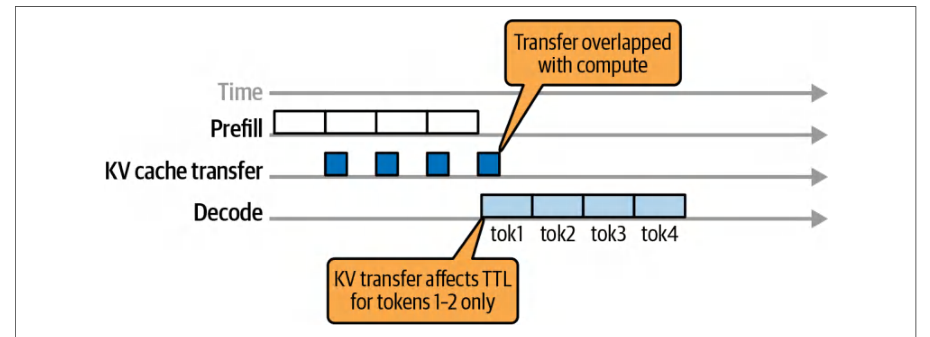
In the prefill stage, the model processes the entire input prompt—often thousands, tens of thousands, or even millions of tokens—in a single forward pass to produce initial hidden states as calculated by the LLM. It then populates the attention key-value (KV) cache for all tokens in the input prompt. Figure 15-1 shows how disaggregated prefill and decode share the KV cache and overlap KV transfers with computations.在预填充阶段，模型在单次前向传播中处理整个输入提示——通常是数千、数万甚至数百万个 token——以产生由 LLM 计算出的初始隐藏状态。随后它为输入提示中的所有 token 填充注意力键值（KV）缓存。图 15-1 展示了解耦预填充与解码如何共享 KV 缓存，并使 KV 传输与计算重叠。

In the decode stage, the model performs an autoregressive generation to predict each new token in the sequence. It does this by consuming the cached attention KV representations of all previously generated tokens.在解码阶段，模型执行自回归生成，以预测序列中的每个新 token。它通过消费所有先前已生成 token 的缓存注意力 KV 表示来完成这一过程。

预填充-解码干扰

Prefill-Decode Interference

Traditionally, LLM inference systems colocate these two stages on the same nodes and simply batch all computations together. However, this naive approach leads to what’s commonly called prefill-decode interference. For instance, a long prompt prefill can occupy the GPU and delay time-sensitive decoding work for other requests—and vice versa.传统上，LLM 推理系统将这两个阶段共置于同一批节点上，并简单地把所有计算合并成批处理。然而，这种朴素做法会导致通常所说的*预填充-解码干扰*。例如，一个长提示词的预填充会占用 GPU，并延迟其他请求中对时延敏感的解码工作——反之亦然。

Colocating prefill and decode on the same nodes forces a single scheduling and resource allocation strategy for these two phases, which have very different characteristics. Prefill consists of large, parallel computations. In contrast, decode requires many small, sequential computations. As a result, systems have to either prioritize one phase’s performance over the other or over-provision hardware to meet both demands.将预填充与解码共置于同一批节点上，会迫使这两个特性迥异的阶段共用同一套调度与资源分配策略。预填充由大规模并行计算构成；相比之下，解码需要大量小规模、串行的计算。因此，系统要么让一个阶段的性能优先于另一个阶段，要么超额配置硬件以满足两者的需求。

With a disaggregated prefill and decode architecture, the prefill and decode phases are assigned to different GPU pools. This eliminates direct interference between the two workloads. The DistServe system, by disaggregating prefill and decode, reported up to 7.4× more goodput requests served within both TTFT and TPOT constraints (up to 12.6× tighter latency SLOs).采用*预填充与解码解耦*架构时，预填充阶段与解码阶段被分配到不同的 GPU 资源池。这消除了两种工作负载之间的直接干扰。DistServe 系统通过解耦预填充与解码，报告称在同时满足 TTFT 与 TPOT 约束的前提下，其服务的有效吞吐请求数最高提升至 7.4 倍（时延 SLO 最多收紧 12.6 倍）。

独立扩展预填充节点与工作节点

Scaling Prefill and Worker Nodes Independently

If we can eliminate cross-phase interference, we can reduce resource “dead time” in which decode tasks are stalled behind long prefill computations—and vice versa. This way, GPUs spend more time doing more useful work and less time idling. This increases utilization and useful throughput at a given latency target (aka goodput).如果能消除跨阶段干扰，我们就能减少资源“死区时间”——即解码任务被长时间的预填充计算阻塞（反之亦然）的时间。这样，GPU 花更多时间做更有用的工作，闲置时间更少。这会提升给定时延目标下的利用率与有用吞吐量（即*有效吞吐*）。

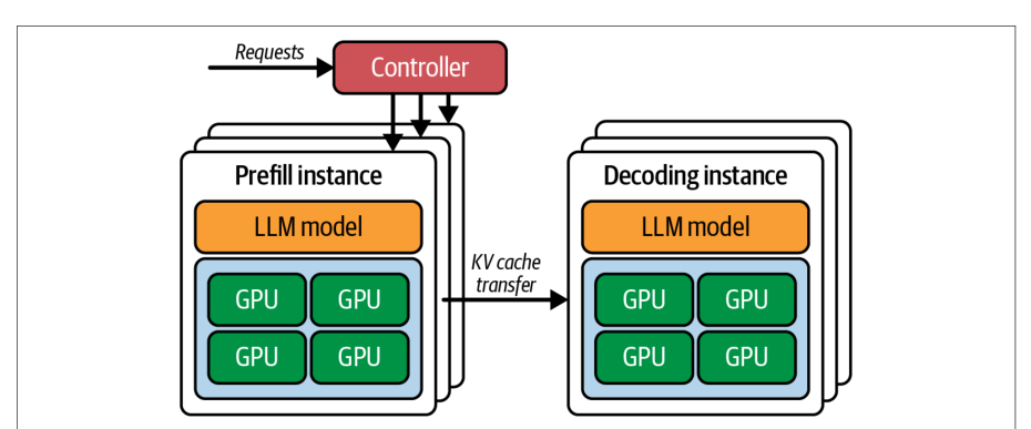
We can scale prefill and decode separately by dedicating one set of nodes to handle the prefill and another set of nodes to handle the decode. The two clusters communicate only when transferring the encoded prompt state, or attention KV cache, from the prefill workers to the decode workers, as shown in Figure 15-2.我们可以通过将一组节点专用于处理预填充、另一组节点专用于处理解码，来分别扩展预填充与解码。两个集群仅在把编码后的提示词状态（即注意力 KV 缓存）从预填充工作节点传输到解码工作节点时通信，如图 15-2 所示。

Here, you see separate GPU workers handling the prefill stage to process the input prompt—along with the decode stage to generate output tokens iteratively. The output of the prefill stage includes the KV cache for the prompt. It is transferred to the decode workers to generate the next tokens.在这里，可以看到独立的 GPU 工作节点负责预填充阶段以处理输入提示词，同时由解码阶段迭代生成输出 token。预填充阶段的输出包含该提示词的 KV 缓存，它被传输到解码工作节点以生成后续 token。

By dedicating separate GPU pools, the system keeps both prefill and decode pipelines busy in parallel. In practice, disaggregation has been shown to significantly improve throughput under strict latency constraints. Some studies show that large gains are possible, but results range from moderate improvements to several times higher goodput once the prefill and decode stages are separated. The results greatly depend on the workload and network fabric.通过专用独立的 GPU 资源池，系统可让预填充与解码两条流水线并行保持忙碌。在实践中，解耦已被证明能在严格的时延约束下显著提升吞吐量。一些研究表明可以获得大幅收益，但一旦将预填充与解码阶段分离，结果从适度改善到有效吞吐提升数倍不等。结果在很大程度上取决于工作负载与网络结构。

This separation allows each stage to be optimized and scaled independently for throughput or latency. Prefills can be batched aggressively on the prefill GPUs to maximize throughput without burdening the decode performance (e.g., increased decode latency). Also, with separate clusters we can tune parallelism settings, instance counts, and scheduling policies specific to each phase.这种分离使每个阶段都能针对吞吐量或时延独立优化与扩展。可以在预填充 GPU 上对预填充进行激进的批处理以最大化吞吐量，而不会拖累解码性能（例如增加解码时延）。此外，借助独立的集群，我们可以针对每个阶段分别调优并行设置、实例数量与调度策略。

对时延（TTFT）与吞吐量（TPOT）的影响

Impact on Latency (TTFT) and Throughput (TPOT)

Decode GPUs can run at lower batch sizes—or with specialized scheduling—to minimize time per output token (TPOT) for streaming generation. For example, you can use a scheduler that prioritizes urgent decode tasks to avoid queuing delays.解码 GPU 可以以较小的批大小运行——或采用专门的调度——以最小化流式生成的*每输出 token 时间*（TPOT）。例如，可以使用优先处理紧急解码任务的调度器来避免排队时延。

This separation works well because each phase has different performance expectations. Time to first token (TTFT) for the prefill stage is optimized for low latency, while the decode stage prioritizes low time per output token (TPOT) and stable streaming latency. End-to-end throughput is largely determined by concurrency and scheduling. In traditional setups, one had to compromise between TTFT and TPOT per-token latency. Disaggregation allows both SLO targets to be met simultaneously.这种分离之所以行之有效，是因为每个阶段有着不同的性能预期。预填充阶段的*首 token 时延*（TTFT）以低时延为优化目标，而解码阶段则优先追求较低的每输出 token 时延（TPOT）和稳定的流式时延。端到端吞吐量在很大程度上由并发度和调度决定。在传统部署中，人们不得不在 TTFT 与 TPOT 的每 token 时延之间做出折中。解耦则允许同时满足这两个 SLO 目标。

The KV handoff incurs minimal additional latency because the communication uses high-bandwidth interconnects for multi-GPU and multinode transfers. These interconnects include NVLink, NVSwitch, InfiniBand, and Ethernet (RoCE on Ethernet) using GPUDirect RDMA. For instance, multinode clusters with ConnectX-8 SuperNICs (800 GbE-class) provides up to 800 Gb/s per port with GPUDirect RDMA. This greatly reduces KV transfer time compared to host-mediated communication paths. Additionally, it’s recommended to deploy 1 NIC per GPU to optimize prefill-decode disaggregation and improve MoE all-to-all performance.KV 交接只会引入极小的额外时延，因为该通信在多 GPU 和多节点传输中使用高带宽互连。这些互连包括 NVLink、NVSwitch、InfiniBand，以及基于 GPUDirect RDMA 的以太网（以太网上的 RoCE）。例如，配备 ConnectX-8 SuperNIC（800 GbE 级）的多节点集群通过 GPUDirect RDMA 可提供每端口高达 800 Gb/s 的带宽。与经由主机中转的通信路径相比，这大幅缩短了 KV 传输时间。此外，建议为每块 GPU 部署 1 个 NIC，以优化预填充-解码解耦并提升 MoE all-to-all 性能。

KV 缓存数据传输与 NIXL

KV Cache Data Transfer and NIXL

Disaggregated systems use a connector or scheduler to transfer the prompt’s intermediate results (the final hidden state and the KV cache) from the prefill workers to the decode workers once the prompt processing is done. This handoff incurs some communication overhead, but if the cluster’s interconnect is high-bandwidth (e.g., NVLink or InfiniBand), this overhead is small compared to the gains from eliminating resource contention.解耦系统使用连接器或调度器，在提示词处理完成后，将提示词的中间结果（最终隐藏状态和 KV 缓存）从预填充工作节点传输到解码工作节点。这种交接会带来一定的通信开销，但如果集群互连是高带宽的（例如 NVLink 或 InfiniBand），那么与消除资源争用所带来的收益相比，这一开销微不足道。

In practice, NVIDIA’s NIXL library minimizes transfer overhead by selecting NVLink/NVSwitch, RDMA, or host-staged paths automatically based on topology and policy. For example, NVIDIA’s NIXL library, introduced in Chapter 4, will automatically select the fastest available path to transmit the KV cache. NIXL integrates with frameworks and inference engines, including Dynamo and vLLM. The NIXL-vLLM integration is shown in Figure 15-3.在实践中，NVIDIA 的 NIXL 库会根据拓扑和策略自动选择 NVLink/NVSwitch、RDMA 或主机暂存路径，从而将传输开销降至最低。例如，第 4 章介绍的 NVIDIA NIXL 库会自动选择可用的最快路径来传输 KV 缓存。NIXL 可与多种框架和推理引擎集成，包括 Dynamo 和 vLLM。NIXL 与 vLLM 的集成如图 15-3 所示。

Specifically, LMCache and NIXL are integrated in vLLM’s disaggregated prefilling as the supported path. NIXL is also used by NVIDIA Dynamo and TensorRT-LLM to transport KV cache data using peer-to-peer GPU interconnects and RDMA.具体而言，LMCache 和 NIXL 已集成到 vLLM 的解耦预填充中，作为受支持的路径。NVIDIA Dynamo 和 TensorRT-LLM 也使用 NIXL，通过 GPU 点对点互连和 RDMA 来传输 KV 缓存数据。

Within a node, NIXL performs device-to-device transfers over NVLink and NVSwitch without host staging. Across nodes, NIXL uses GPUDirect RDMA over InfiniBand or RoCEv2 to avoid host copies. These paths keep KV cache handoff latency low even for multigigabyte payloads.在节点内部，NIXL 通过 NVLink 和 NVSwitch 执行设备到设备传输，无需主机暂存。跨节点时，NIXL 使用基于 InfiniBand 或 RoCEv2 的 GPUDirect RDMA 来避免主机拷贝。即便负载达到数 GB，这些路径也能让 KV 缓存交接保持低时延。

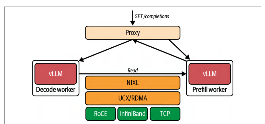
Placement of prefill and decode workers should follow the fabric. Same node placement keeps KV transfers on NVLink and NVSwitch via CUDA peer access, while cross-node placement should use GPUDirect RDMA over InfiniBand or RoCEv2. NVIDIA Dynamo integrates with NIXL to move KV cache between GPUs, CPU memory, and storage across nodes, and vLLM integrates through LMCache and NIXL for disaggregated prefilling.预填充和解码工作节点的部署位置应遵循网络架构。同节点部署通过 CUDA 点对点访问让 KV 传输走 NVLink 和 NVSwitch；跨节点部署则应使用基于 InfiniBand 或 RoCEv2 的 GPUDirect RDMA。NVIDIA Dynamo 与 NIXL 集成，可在跨节点的 GPU、CPU 内存和存储之间搬运 KV 缓存；vLLM 则通过 LMCache 和 NIXL 集成来实现解耦预填充。

使用 Kubernetes 部署解耦的预填充与解码

Deploying Disaggregated Prefill and Decode with Kubernetes

In an advanced deployment, a cluster orchestration system like Kubernetes can dynamically shift the GPU pool allocations—or scale the pools out separately—based on load and input characteristics. For instance, if many users arrive with superlong prompts and relatively small outputs (e.g., large-document summarization use cases), Kubernetes can temporarily shift the allocation to use more GPUs in the prefill pool. This will decrease the number of GPUs allocated to the decode phase.在高级部署中，像 Kubernetes 这样的集群编排系统可以根据负载和输入特征动态调整 GPU 池的分配——或者分别对各个池进行横向扩容。例如，如果大量用户带来超长提示词和相对较小的输出（例如大文档摘要用例），Kubernetes 可以临时倾斜分配，让预填充池使用更多 GPU。这会减少分配给解码阶段的 GPU 数量。

In contrast, if many users arrive requesting superlong outputs (e.g., long reasoning chains, “think step-by-step,” etc.), more GPUs can be shifted to the decode pool. In both cases, new instances can be scaled out for each worker type.相反，如果大量用户请求超长输出（例如长推理链、“逐步思考”等），则可以将更多 GPU 转移到解码池。在这两种情况下，都可以为每种工作节点类型横向扩容新的实例。

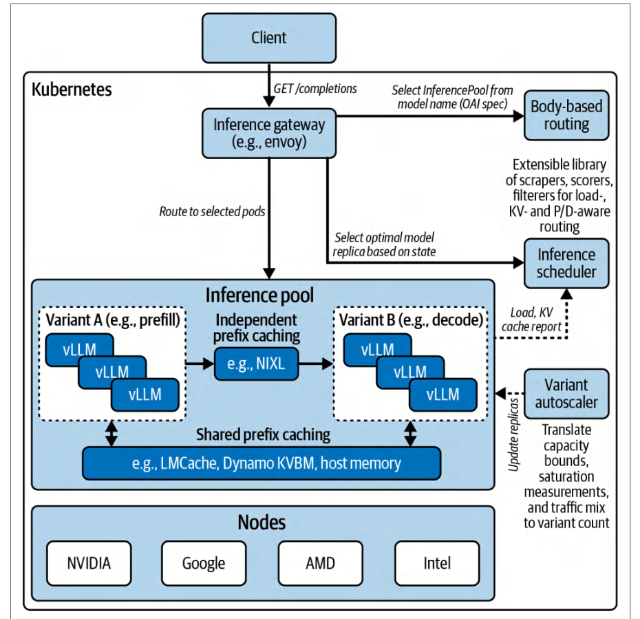
Figure 15-4 shows a distributed, Kubernetes-based vLLM cluster of separate prefill and decode workers using the open source llm-d project. vLLM implements disaggregated prefilling by running two instances and handing off KV using LMCache and NIXL, but llm-d extends this with Kubernetes native orchestration for disaggregated serving and KV-aware routing. This diagram shows a component called the variant autoscaler, which is responsible for updating the number of replicas for the prefill and decode workers in the pool.图 15-4 展示了一个基于 Kubernetes 的分布式 vLLM 集群，使用开源 llm-d 项目将预填充与解码工作节点分离。vLLM 通过运行两个实例并使用 LMCache 和 NIXL 交接 KV 来实现解耦预填充，而 llm-d 在此基础上进一步扩展，提供了面向解耦服务的 Kubernetes 原生编排和 KV 感知路由。该图展示了一个名为 variant autoscaler 的组件，它负责更新池中预填充与解码工作节点的副本数量。

Overall, a disaggregated prefill/decode architecture provides a foundation for high-throughput, low-latency LLM serving. It does introduce complexity, however, as intermediate data must be transferred and managed—on the order of a few gigabytes for the KV cache of a long prompt. And scheduling is more involved, but the benefits of utilizing hardware efficiently are significant at ultra scale.总体而言，解耦的预填充/解码架构为高吞吐、低时延的 LLM 服务提供了基础。不过它确实引入了复杂性，因为必须传输和管理中间数据——对于长提示词的 KV 缓存，其规模可达数 GB。调度也更加复杂，但在超大规模下，高效利用硬件所带来的收益是显著的。

服务超大规模 MoE 模型的并行策略

Parallelism Strategies for Serving Massive MoE Models

Serving massive MoE models efficiently requires multiple forms of parallelism due to limited GPU memory. We break down the key parallelism strategies, including tensor, pipeline, expert, data, and context parallel. We’ll also discuss how they can be combined to distribute an LLM across many GPUs. Table 15-1 provides a high-level summary of these strategies, their typical use, and a description of each strategy in more detail as they relate to inference.高效服务超大规模 MoE 模型需要多种形式的并行，因为 GPU 显存有限。我们逐一剖析关键的并行策略，包括张量并行、流水线并行、专家并行、数据并行和上下文并行。我们还将讨论如何将它们组合起来，把一个 LLM 分布到众多 GPU 上。表 15-1 对这些策略、其典型用途以及每种策略在与推理相关方面的更详细描述做了高层总结。

Parallelism strategy并行 策略

Partition basis Use case Pros Cons划分依据 用例 优点 缺点

Tensor parallelism张量并行

Within each layer (split neural network weight matrices across GPUs)在每一层内部（将神经网络权重矩阵拆分到多个 GPU 上）

Single model is too large or you need to speed up heavy compute within layers across multiple GPUs单个模型过大，或者需要跨多个 GPU 加速层内的高强度计算

Near-linear speedup on compute-bound layers Reduced overhead due to overlapping all-reduce communication with computation在计算受限层上获得接近线性的加速 通过将 all-reduce 通信与计算重叠来降低开销

Frequent communication at each layer (all-reduce) Requires high-bandwidth interconnect (NVLink/NVSwitch) Less efficient across nodes and slow networks due to high latencies (Recommended to keep tensor parallel groups within a single node)每一层都有频繁通信（all-reduce） 需要高带宽互连（NVLink/NVSwitch） 跨节点及慢速网络下因高时延而效率较低（建议将张量并行组保持在单个节点内）

Parallelism strategy并行 策略

Partition basis Use case Pros Cons划分依据 用例 优点 缺点

Pipeline parallelism流水线并行

Different layers on different GPUs (the model is sliced by layer sequence)不同层位于不同 GPU 上（模型按层顺序切分）

Extremely deep models that don’t fit on one GPU Memory scaling across layers无法放入单个 GPU 的超深模型 跨层的显存扩展

Allows distribution of model state Uses microbatching to process multiple tokens from different users/requests concurrently Multiple layers can be processed in parallel for long sequences (improves throughput for large batches or long inputs)允许分布模型状态 使用微批处理并发处理来自不同用户/请求的多个 token 对于长序列，多层可并行处理（提升大批量或长输入的吞吐量）

Adds pipeline fill/flush latency (bubbles)—not helpful for one-token-at-a-time decoding More complex to implement and higher activation memory footprint (must store intermediate activations between pipeline stages)引入流水线填充/排空时延（气泡）——对逐 token 解码没有帮助 实现更复杂，且激活显存占用更高（必须在流水线各级之间存储中间激活）

Expert parallelism专家并行

Different MoE on different GPUs (sparse activation per token)不同 MoE 位于不同 GPU 上（每个 token 稀疏激活）

Massive MoE models with many experts Needed to shard model parameters across GPUs拥有大量专家的超大规模 MoE 模型 需要将模型参数分片到多个 GPU 上

Enables virtually unlimited model size—total parameters scale with number of GPUs Each GPU computes only a fraction of tokens (sparse compute) High parameter count boosts model capacity/quality使模型规模几乎不受限制——总参数量随 GPU 数量扩展 每个 GPU 只计算一小部分 token（稀疏计算） 高参数量提升模型容量/质量

High runtime communication overhead (all-to-all) at each MoE layer Potential load imbalance if gating is uneven Each GPU must have enough work (tokens) per expert to amortize communication每个 MoE 层在运行时都有较高的全对全（all-to-all）通信开销 若门控不均衡，可能出现负载不均衡 每个 GPU 上每个专家必须有足够的工作量（token）以摊薄通信开销

Data parallelism数据并行

Replicate the entire model on multiple GPUs, serving different requests on each在多块 GPU 上复制整个模型，每块 GPU 服务不同的请求

No latency improvement for individual queries (aka per-query latency) Multiplies memory usage (each replica uses full memory) Must handle consistency if stateful (e.g., caches) or use stateless model calls Context parallelism对单个查询（即*每查询* 时延）没有时延改善；显存占用成倍增加（每个副本都使用完整内存）；若为有状态（例如缓存）则必须处理一致性问题，或改用无状态的模型调用。上下文并行

Scaling out throughput (more concurrent requests) once model deployment is fixed Multi-instance serving for many users在模型部署固定后横向扩展吞吐量（更多并发请求）；面向多用户的多实例服务

Nearly linear throughput scaling Simple to implement (no model partitioning needed)吞吐量近乎线性扩展；实现简单（无需对模型分区）

Partition the input sequence tokens across GPUs at each layer在每一层将输入序列的 token 划分到多块 GPU 上

Ultralong sequences (e.g., 100k+ tokens) to reduce prompt latency and memory per GPU适用于超长序列（例如 100k+ token），以降低提示时延和每块 GPU 的显存占用

Achieves near-linear speedup for long context prefill Enables processing contexts that exceed one GPU’s memory by splitting KV cache对长上下文预填充实现近乎线性的加速；通过拆分 KV 缓存，可处理超出单块 GPU 显存的上下文

Requires custom attention algorithms to handle attention across partitions Adds communication per layer for boundary tokens Beneficial for very long contexts (100k+ tokens) due to additional communication overhead需要自定义注意力算法来处理跨分区的注意力；每层都会为边界 token 增加通信；由于额外的通信开销，仅对超长上下文（100k+ token）才有收益

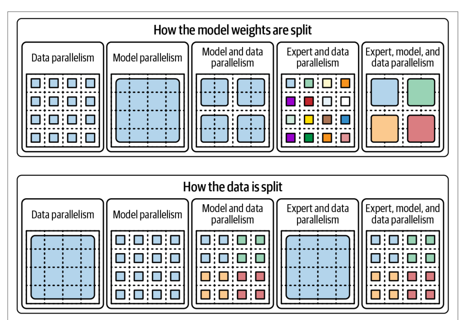
These parallelism strategies define how the model weights and data are split over the GPUs. Figure 15-5 shows how they are split up for the different parallelism strategies— as well as common combinations of strategies.这些并行策略定义了模型权重与数据如何在多块 GPU 上切分。图 15-5 展示了在不同并行策略下它们是如何切分的，以及常见的策略组合。

张量并行

Tensor Parallelism

Tensor parallelism (TP) splits the computations within each layer of the neural network across multiple GPUs. For instance, a large matrix multiply in a transformer layer can be partitioned by columns or rows—and computed in parallel on two or more GPUs. These GPUs then exchange their results by performing an all-reduce to aggregate their partial outputs.张量并行（TP）将神经网络每一层内的计算拆分到多块 GPU 上。例如，Transformer 层中的大型矩阵乘法可以按列或按行划分，并在两块或多块 GPU 上并行计算。随后这些 GPU 通过执行全归约来交换结果，以聚合各自的部分输出。

TP is commonly used when a model’s layers, called hidden layers, are too large to fit into a single GPU’s memory—or when we want to accelerate a single instance of a model by utilizing multiple GPUs for the same layer in parallel. It keeps all GPUs in lockstep for each layer’s computation, which requires extremely high inter-GPU bandwidth to be efficient.当模型的层（称为*隐藏层*）过大而无法放入单个 GPU 的内存时，或者当我们希望利用多个 GPU 并行处理同一层来加速模型的单个实例时，通常会使用 TP。它让所有 GPU 在每一层的计算上保持锁步，这要求极高的 GPU 间带宽才能高效。

Ideally, TP runs on GPUs that are connected with high-bandwidth NVLink and NVSwitch interconnects. On multi-GPU Blackwell systems that use fifth-generation NVLink (up to 1.8 TB/s aggregate bidirectional GPU-to-GPU bandwidth and advanced network topologies), TP can scale efficiently across a node of 8–16 GPUs— or even up to 72 GPUs in the case of an NVL72 rack. Remember, within the GB200/ GB300 NVL72 racks, NVLink Switch provides about 130 TB/s of aggregate GPU bandwidth within the 72 GPU domain. This is a large amount of intra-rack bandwidth.理想情况下，TP 运行在通过高带宽 NVLink 与 NVSwitch 互连连接的 GPU 上。在使用第五代 NVLink（聚合双向 GPU 间带宽最高 1.8 TB/s，并具备先进的网络拓扑）的多 GPU Blackwell 系统上，TP 可以在一个 8–16 GPU 的节点内高效扩展——在 NVL72 机架的情况下甚至可以扩展到 72 个 GPU。请记住，在 GB200/GB300 NVL72 机架内，NVLink Switch 在 72 GPU 域内提供约 130 TB/s 的聚合 GPU 带宽。这是相当大的机架内带宽。

TP provides near-linear speedups for compute-bound portions of the model as long as collective communications, such as the all-reduce of activations, are fast relative to computation. In inference, tensor parallelism is mainly applied to the large matrix multiplications of the attention projections and feed-forward multilayer perceptron (MLP) networks.只要集合通信（例如激活值的全归约）相对于计算足够快，TP 就能为模型中受计算限制的部分提供接近线性的加速比。在推理中，张量并行主要应用于注意力投影以及前馈多层感知机（MLP）网络中的大型矩阵乘法。

Since the activations for one token are relatively small, those all-reduce communications are not too costly on NVLink. As such, TP is a common strategy for splitting giant dense models across GPUs without approximating model weights.由于单个 token 的激活值相对较小，这些全归约通信在 NVLink 上的开销并不算高。因此，TP 是一种常见的策略，用于将巨型稠密模型拆分到多个 GPU 上，而无需对模型权重做近似。

We mainly use TP to serve models in which single MoE experts or transformer layers are too large for a single GPU. However, we also use it when we want to reduce latency by parallelizing each layer’s computations across multiple GPUs.我们主要使用 TP 来服务那些单个 MoE 专家或 Transformer 层对单个 GPU 而言过大的模型。不过，当我们希望通过将每一层的计算并行到多个 GPU 上来降低时延时，也会使用它。

One must be mindful that beyond a certain scale, however, TP efficiency drops— especially when using it across nodes or racks running over InfiniBand or Ethernet. In practice, it’s best to use TP for intranode communication—or between nodes in an NVLink domain.但必须注意，超过一定规模后，TP 的效率会下降——尤其是在跨节点或跨机架、通过 InfiniBand 或以太网运行时。在实践中，最好将 TP 用于节点内通信——或用于 NVLink 域内的节点之间。

Modern multi-GPU racks like NVIDIA’s GB200/GB300 NVL72 allow TP to be used at a much larger scale without saturating interconnect bandwidth. NVLink Switch extends the NVLink domain across the rack to 72 GPUs per NVL72. NVLink Switch Systems can scale an all-to-all, fully connected NVLink fabric across up to 8 racks, or 576 GPUs (576 GPUs = 8 racks * 72 GPUs per rack). This enables large-scale parallelism strategies, not just inside a single NVL72 but also across multiple racks. For instance, in an 8-rack topology, you can increase to 576-way tensor parallelism using the 576 GPUs across 8 racks (576 GPUs = 8 racks × 72 GPUs per rack.)像 NVIDIA GB200/GB300 NVL72 这样的现代多 GPU 机架，使 TP 能够在更大规模上使用而不会打满互连带宽。NVLink Switch 将 NVLink 域扩展到整个机架，每个 NVL72 可达 72 个 GPU。NVLink Switch 系统可以将全互联、完全连接的 NVLink 网络结构扩展到最多 8 个机架，即 576 个 GPU（576 个 GPU = 8 个机架 * 每个机架 72 个 GPU）。这不仅能在单个 NVL72 内部、还能跨多个机架实现大规模并行策略。例如，在 8 机架拓扑中，你可以利用跨 8 个机架的 576 个 GPU 提升到 576 路张量并行（576 个 GPU = 8 个机架 × 每个机架 72 个 GPU）。

流水线并行

Pipeline Parallelism

Pipeline parallelism (PP) partitions the model layer-wise across different GPUs. For example, in a 60-layer transformer-based model, GPU 0 might hold layers 1–20, GPU 1 holds layers 21–40, and GPU 2 holds layers 41–60.流水线并行（PP）将模型*按层*划分到不同的 GPU 上。例如，在一个 60 层的 Transformer 模型中，GPU 0 可能持有第 1–20 层，GPU 1 持有第 21–40 层，GPU 2 持有第 41–60 层。

When processing a sequence of tokens, the data flows through the GPUs in sequence such that GPU 0 computes layers 1–20, then passes its intermediate activations to GPU 1 for layers 21–40, and so on. This allows models that are too deep to fit on one accelerator to be distributed.在处理一个 token 序列时，数据依次流经各个 GPU：GPU 0 计算第 1–20 层，然后将其中间激活值传给 GPU 1 以计算第 21–40 层，依此类推。这使得因过深而无法放入单个加速器的模型得以分布式部署。

In inference, PP can improve throughput by partitioning the model across multiple batches—similar to an assembly line. During the prefill phase, which processes a long sequence of input tokens, PP achieves high GPU utilization by streaming different portions of the sequence into the layers in staggered fashion.在推理中，PP 可以通过将模型划分到多个批次上来提升吞吐量——类似于一条装配线。在*预填充*阶段（该阶段处理一长串输入 token），PP 以交错的方式将序列的不同部分送入各层，从而实现较高的 GPU 利用率。

In contrast, during the decode phase, generating one token at a time, pure PP offers less benefit since each new token must still pass through the pipeline stages sequentially. This creates pipeline bubbles, or idle periods, in which earlier stages wait for later ones to finish for each and every token.相比之下，在*解码*阶段，每次只生成一个 token，纯 PP 带来的收益较小，因为每个新 token 仍必须依次经过各个流水线阶段。这会产生流水线气泡（即空闲期），在此期间，对每一个 token，靠前的阶段都要等待靠后的阶段完成。

To reduce pipeline bubbles, implementations use microbatching, which allows the pipeline to process multiple tokens from different requests concurrently. Still, pipeline parallelism primarily helps with memory scaling by enabling very large models to split layers among GPUs. It also helps throughput—especially when handling large batch sizes or long inputs.为减少流水线气泡，实现中会采用微批处理（microbatching），使流水线能够并发处理来自不同请求的多个 token。不过，流水线并行主要有助于内存扩展，因为它能让超大模型把层拆分到多块 GPU 上。它也有助于提升吞吐量——尤其是在处理大批大小或长输入时。

PP tends to increase end-to-end latency for a single item due to transfer overhead between pipeline stages. As such, PP is usually chosen for model capacity reasons— rather than latency reasons. This is because it can fit the model into memory. The slight latency hit is acceptable when no single GPU can hold the whole model.由于流水线各阶段之间的传输开销，PP 往往会增加单个条目的端到端时延。因此，选择 PP 通常是出于模型容量的考虑，而非时延的考虑，因为它能把模型装进内存。当没有任何单块 GPU 能容纳整个模型时，这点轻微的时延损失是可以接受的。

Additionally, PP is often used in combination with other parallelism strategies like TP to balance memory and speed. When serving large MoE models, one might use pipeline parallelism across 2–4 GPUs to split the deep layer stack—while relying on TP to handle the wide, intralayer compute.此外，PP 常与其他并行策略（如 TP）结合使用，以平衡内存与速度。在服务大型 MoE 模型时，可以用跨 2–4 块 GPU 的流水线并行来拆分深层堆栈，同时依靠 TP 处理层内的大规模计算。

专家并行

Expert Parallelism

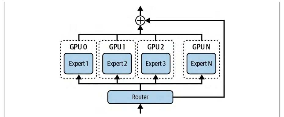
Expert parallelism (EP) is specific to MoE architectures. In an MoE layer, there are many expert networks, or feed-forward sublayers. For each input token, only one or a few experts are activated. This naturally lends itself to distributing different experts on different GPUs.专家并行（EP）是 MoE 架构特有的。在一个 MoE 层中有许多专家网络，即前馈子层。对每个输入 token，只有一或少数几个专家被激活。这天然适合把不同的专家分布到不同的 GPU 上。

For instance, if an MoE layer has 16 experts and we have 4 GPUs, each GPU could host 4 experts. During inference, when a token arrives at that MoE layer, its internal gating network will choose the top two experts, for instance, for that token. The token’s data is then sent to whichever GPUs own those two experts for processing. Then the results are combined back to generate the next token, as shown in例如，若一个 MoE 层有 16 个专家，而我们有 4 块 GPU，则每块 GPU 可承载 4 个专家。推理时，当一个 token 到达该 MoE 层，其内部的门控网络会为该 token 选择前两个专家（举例而言）。随后该 token 的数据被发送到拥有这两个专家的 GPU 上处理，结果再被合并回来以生成下一个 token，如图所示。

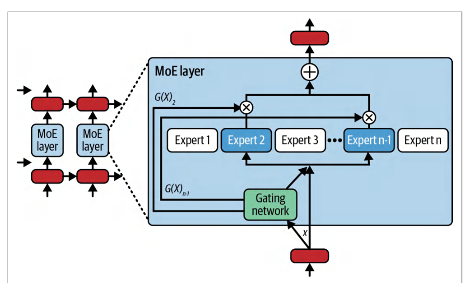
Implementing this requires an all-to-all communication pattern such that tokens (technically, their activation vectors) are dynamically shuffled between GPUs so that each token lands on the GPU of its assigned expert. After each expert computes its output for its assigned tokens, another all-to-all is performed to return the token outputs back to their original order.实现这一点需要全对全（all-to-all）通信模式，使 token（严格说是其激活向量）在 GPU 之间动态重排，从而让每个 token 落到其被分配专家的那块 GPU 上。每个专家为其分到的 token 计算完输出后，再执行一次全对全通信，把 token 的输出按原始顺序送回。

This dynamic routing introduces a communication-heavy step at each MoE layer. This can become a performance bottleneck if not carefully optimized—especially as the number of experts/GPUs increases. The upside is that expert parallelism allows the total model capacity to scale almost linearly with the number of GPUs.这种动态路由在每个 MoE 层都引入了一个通信密集的步骤。若不加仔细优化，它可能成为性能瓶颈——尤其是随着专家/GPU 数量增加时。好处是，专家并行使模型总容量几乎能随 GPU 数量线性扩展。

Consider an MoE with 100 experts distributed across 100 GPUs. If each token activates only two experts, the compute per token is similar to a smaller dense model. As such, expert parallelism is what allows some massive MoE models to be served at all since the model weights are sharded across many GPUs—and each GPU handles only a fraction of the tokens at any given layer.设想一个 MoE 有 100 个专家，分布在 100 块 GPU 上。若每个 token 只激活两个专家，则每个 token 的计算量相当于一个更小的稠密模型。正因如此，专家并行才使某些超大规模 MoE 模型得以被服务：模型权重分片到许多 GPU 上，而在任意给定层上，每块 GPU 只处理一小部分 token。

Efficient expert parallel inference requires careful load balancing—as well as high-bandwidth interconnects, such as NVLink/NVSwitch for intra-rack communication and InfiniBand/RDMA for internode communication. Modern MoE inference frameworks use fast collective communication libraries like NCCL. It often helps to group multiple experts per GPU to reduce communication steps.高效的专家并行推理需要谨慎的负载均衡，还需要高带宽互连，例如用于机架内通信的 NVLink/NVSwitch 和用于节点间通信的 InfiniBand/RDMA。现代 MoE 推理框架使用 NCCL 这类高速集合通信库。通常，把多个专家分组到同一块 GPU 上以减少通信步骤会很有帮助。

Modern MoE inference often uses top-2 gating, in which each token is assigned to two experts. To reduce communication, you can group commonly paired experts onto the same GPU or compute node. For instance, if tokens use two experts, placing those two frequently paired experts on the same GPU or node means that many token assignments will stay on a single GPU or node, which will localize communication traffic and reduce overhead.现代 MoE 推理常采用 top-2 门控（top-2 gating），即每个 token 被分配给两个专家。为减少通信，可以把经常成对出现的专家分组到同一块 GPU 或同一个计算节点上。例如，如果 token 使用两个专家，那么把这两个频繁配对的专家放在同一块 GPU 或同一个节点上，意味着许多 token 分配会留在单块 GPU 或单个节点内，从而将通信流量本地化并降低开销。

Another technique is to use top-1 gating, in which each token goes to only one expert. This will reduce the communication volume relative to top-2 gating described previously, which doubles the number of expert outputs. While top-1 gating is faster, it can lead to a lower model quality and uneven load.另一种技术是采用 top-1 门控，即每个 token 只发送到一个专家。与前面描述的 top-2 门控相比，这会减少通信量——top-2 门控会使专家输出数量翻倍。虽然 top-1 门控更快，但可能导致模型质量下降和负载不均。

Many MoE LLMs use at least top-2 gating for better quality, good speed, and balanced load. Additionally, it’s important to place experts strategically—or even use backup expert replicas to avoid overloading experts.许多 MoE LLM 至少采用 top-2 门控，以获得更好的质量、良好的速度和均衡的负载。此外，策略性地放置专家——甚至使用备用专家副本以避免专家过载——也很重要。

When experts become overloaded, or hot, they can become throughput bottlenecks if the gating network is disproportionately routing tokens to them. The straggler effect, as it’s called, requires that all expert computations be complete before they can progress. As such, an overloaded expert that receives more work (tokens) than other experts will stall the inference pipeline. This will leave some experts, and their GPUs, idle while the other experts catch up.当专家过载（变“热”）时，如果门控网络不成比例地将 token 路由给它们，它们就会成为吞吐量瓶颈。所谓的*掉队者效应*（straggler effect）要求所有专家计算都完成后才能继续推进。因此，接收比其他专家更多工作（token）的过载专家会拖住推理流水线。这会导致部分专家及其 GPU 处于空闲状态，等待其他专家追赶上来。

To prevent this, high-performance MoE serving systems expose a capacity factor parameter, typically set at 1.2–1.5× the average token load, which caps how many tokens each expert can process per batch. Tokens beyond that are routed to a second-choice overflow expert—or queued for a second pass. This complements any load-balancing loss or gating noise used during training to encourage the MoE to assign tokens to experts uniformly.为防止这种情况，高性能 MoE 服务系统会暴露一个容量因子参数，通常设为平均 token 负载的 1.2–1.5 倍，用以限制每个专家每批可处理的 token 数量。超出该上限的 token 会被路由到次选溢出专家——或排队等待第二轮处理。这与训练期间使用的任何负载均衡损失或门控噪声相辅相成，促使 MoE 将 token 均匀分配给各专家。

Some full-featured inference servers can also replicate hot experts onto multiple GPUs to split the load if necessary. This comes at a cost of additional GPU memory. We will see an example of load imbalance a bit later.一些功能完备的推理服务器还可以在必要时将热门专家复制到多块 GPU 上以分摊负载。代价是额外的 GPU 显存。稍后我们会看到一个负载不均衡的例子。

The combination of inference-time spillover (capacity factor), training-time penalties (load-balancing loss and gating noise), and hot-expert replicas should smooth out the token-expert load distribution when capacity is reached—maximizing overall MoE inference throughput.推理时的溢出（容量因子）、训练时的惩罚（负载均衡损失和门控噪声）以及热门专家副本三者结合，应在达到容量时平滑 token 与专家之间的负载分布——从而最大化 MoE 推理的整体吞吐量。

数据并行

Data Parallelism

In inference, data parallelism (DP) refers to replicating the entire model on multiple GPUs and assigning different incoming requests—or shards of a request batch—to each GPU. Unlike data parallelism in training, which keeps models in sync with gradient averaging, data parallelism in inference runs independent forward passes on each replica. This is the simplest way to scale out throughput.在推理中，数据并行（DP）指将整个模型复制到多块 GPU 上，并把不同的传入请求——或请求批次的分片——分配给每块 GPU。与训练中通过梯度平均保持模型同步的数据并行不同，推理中的数据并行在每个副本上运行独立的前向传播。这是扩展吞吐量最简单的方式。

For instance, with DP, if one GPU can handle 10 requests per second, using 8 GPUs with 8 replicas ideally gives 80 requests per second of throughput—assuming the requests are independent. In practice, using data parallelism for inference requires spinning up multiple model-serving engines and load-balancing requests among them.例如，在 DP 下，如果一块 GPU 每秒能处理 10 个请求，那么使用 8 块 GPU 构成 8 个副本，理想情况下可获得每秒 80 个请求的吞吐量——前提是这些请求彼此独立。在实践中，用数据并行做推理需要启动多个模型服务引擎，并在它们之间对请求做负载均衡。

When using DP, each GPU, or group of GPUs, handles a subset of queries from start to finish. The advantage is linear scaling of throughput and no inter-GPU communication during inference since each replica runs in isolation. The disadvantages are significant, however.使用 DP 时，每块 GPU（或每组 GPU）从头到尾处理一部分查询。其优势是吞吐量线性扩展，且由于每个副本独立运行，推理期间没有 GPU 间通信。然而其劣势也相当显著。

DP multiplies the memory requirement since each replica needs a full copy of model weights and cache. As such, serving a model with eight replicas uses 8× the GPU memory—and roughly 8× the hardware cost—compared to hosting the model on a single GPU.DP 会成倍放大显存需求，因为每个副本都需要一份完整的模型权重与缓存副本。因此，与在单块 GPU 上托管模型相比，用 8 个副本服务一个模型会占用 8 倍的 GPU 显存，硬件成本也约为 8 倍。

In practice, data parallelism is often combined with request batching and multistream execution on each GPU to maximize utilization. Each replica should ideally be stateless—or use synchronized caches to avoid consistency issues.在实践中，数据并行常与请求批处理以及每块 GPU 上的多流执行结合使用，以最大化利用率。理想情况下，每个副本应是无状态的——或者使用同步的缓存以避免一致性问题。

It’s important to note that DP does not reduce latency for any single request. It does, however, improve throughput since there are more replicas available to handle requests—assuming the memory and compute resources are available and relatively free of contention.需要强调的是，DP 不会降低任何单个请求的时延。但它确实能提升吞吐量，因为有更多副本可用于处理请求——前提是内存与计算资源充足且基本不存在争用。

For inference, DP is often used in combination with other parallelism approaches, such as TP and PP, due to the additional memory and cost requirements of DP. For example, if a model must be spread across eight GPUs due to memory limitations, it should use DP with TP, PP, or EP—or even all of them together—to create four-dimensional (4D) parallelism (add in context parallelism (CP), and you’re using 5D parallelism!).在推理中，由于 DP 额外的内存与成本需求，它常与其他并行方式（如 TP 和 PP）结合使用。例如，如果由于内存限制必须把一个模型分散到 8 块 GPU 上，就应当把 DP 与 TP、PP 或 EP——甚至全部同时——结合使用，从而构成四维（4D）并行（再加上上下文并行（CP），你用的就是 5D 并行！）。

Specifically, you can use DP with TP to deploy two large, 8-GPU model replicas using two DP groups of eight GPUs. This will double the throughput and shard each of the large model replicas across eight GPUs within its layers using TP.具体来说，你可以用 DP 配合 TP，通过两个各含 8 块 GPU 的 DP 组来部署两个大型的 8-GPU 模型副本。这将使吞吐量翻倍，并利用 TP 在每个大型模型副本的各层内部将其分片到 8 块 GPU 上。

In a massive inference cluster, you can dedicate a large number of GPUs and nodes to serve multiple copies of the large model to handle high request volumes. DP is particularly useful when throughput needs to scale beyond what a single model instance can provide. In practice, production systems often run many DP replicas of the large model to meet traffic demands.在超大规模推理集群中，你可以投入大量 GPU 和节点来服务该大型模型的多个副本，以应对高请求量。当吞吐需求超出单个模型实例所能提供的水平时，DP 尤其有用。在实践中，生产系统常常运行该大型模型的许多 DP 副本来满足流量需求。

上下文（序列）并行

Context (Sequence) Parallelism

Context parallelism (CP) is more of a specialized strategy that partitions a single sequence of tokens across multiple GPUs. This technique benefits extremely long context inputs on the order of tens of thousands and millions of tokens. These would otherwise be too slow or memory-heavy or simply not fit on a single GPU.上下文并行（CP）更像是一种专用策略，它把单个 token 序列划分到多块 GPU 上。该技术适用于数万乃至数百万 token 量级的超长上下文输入——否则这些输入要么太慢、要么显存占用过大，或者根本无法放进单块 GPU。

The idea behind CP is to split the sequence into chunks and have different GPUs handle different parts of the sequence in parallel at each layer. The GPUs exchange only the necessary information at the boundary between chunks of the sequence.CP 的思路是把序列切分成若干块，让不同的 GPU 在每一层并行处理序列的不同部分。GPU 之间只在序列各块的边界处交换必要信息。

CP handles contexts larger than a single GPU’s memory by splitting the KV cache across GPUs. It also reduces prompt-processing latency roughly in proportion to the number of GPUs used. As such, CP can achieve near-linear speedup for very long context prefill runs by using multiple GPUs to perform the prefill for a long context in parallel.CP 通过把 KV 缓存拆分到多块 GPU 上，从而处理超出单块 GPU 显存的上下文。它还能把提示处理的时延大致按所用 GPU 数量成比例地降低。因此，通过使用多块 GPU 并行地对长上下文执行预填充，CP 可以为超长上下文预填充实现接近线性的加速。

The challenge with CP is that transformers have global self-attention such that every token attends to every earlier token. Naively splitting the sequence would require lots of information exchange between GPUs to compute attention across the partition boundary.上下文并行（CP）面临的挑战在于，Transformer 具有全局自注意力，即每个 token 都要关注此前所有的 token。若简单地切分序列，则需要在 GPU 之间进行大量信息交换，以计算跨越分区边界的注意力。

CP methods use clever schemes like ring parallelism and blocked attention to reduce the quadratic self-attention communication time complexity—and limit each GPU to attending mostly within its partition of the context as well as a small amount of chunk-boundary data.CP 方法采用环形并行（ring parallelism）和分块注意力（blocked attention）等巧妙方案，以降低自注意力通信的二次时间复杂度，并使每个 GPU 主要只在其上下文分区内以及少量块边界数据上进行注意力计算。

In effect, each GPU handles a subset of positions in the input sequence for each layer. They pass intermediate results around in a pipelined fashion—often arranged in a ring. CP is analogous to pipeline parallelism but along the sequence-length dimension instead of the layer dimension.实际上，每个 GPU 在每一层处理输入序列中一部分位置。各 GPU 以流水线方式传递中间结果——通常组织成环形。CP 类似于流水线并行，只是沿序列长度维度而非层维度切分。

Context parallelism excels at prefill for very long inputs by slicing a document into segments, allocating segments across multiple GPUs, and processing each segment concurrently. This reduces prompt-processing time roughly in half for every doubling of GPUs—with only a bit of overhead for cross-segment attention at the boundaries.上下文并行在超长输入的预填充阶段表现优异：它将文档切分为若干段，把各段分配到多个 GPU 上并并发处理每一段。GPU 数量每翻一倍，提示词处理时间大约减半——只需为边界处的跨段注意力付出少量开销。

In short, while CP doesn’t speed up the sequential, token-by-token decode phase, it can shorten TTFT for extremely long prompts. It does this by distributing the attention KV cache across devices such that each GPU stores only its segment’s cache. CP also lets you handle contexts larger than what a single GPU can fit into memory.简而言之，CP 虽然无法加速逐 token 的顺序解码阶段，但可以缩短极长提示词的 TTFT。其做法是将注意力的 KV 缓存分布到各设备上，使每个 GPU 只存储自己那一段的缓存。CP 还让你能够处理超出单块 GPU 显存容量的上下文。

混合并行

Hybrid Parallelism

In practice, serving massive MoE LLMs uses a combination of the previous parallelism strategies. Today’s LLM models are so large and complex that no single parallelization method is sufficient. Figure 15-7 shows a hybrid parallel configuration using four GPUs.在实践中，服务大规模 MoE LLM 需要组合使用前面介绍的多种并行策略。如今的 LLM 模型规模庞大且结构复杂，单一并行方法已不足以应对。图 15-7 展示了一个使用四块 GPU 的混合并行配置。

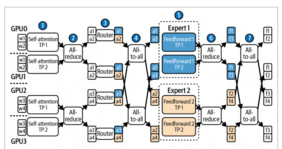
Here, we are using four pipeline stages (one per GPU) and two-way tensor parallelism. The tokens are routed across two experts using expert parallelism. This is called a 4 × 2 EP hybrid parallel strategy.这里我们使用四个流水线阶段（每块 GPU 一个）和两路张量并行。token 通过专家并行在两位专家之间路由。这被称为 4 × 2 EP 混合并行策略。

Let’s go even larger and create logic groups of GPUs. For example, consider a cluster of 64 GPUs. We can group the GPUs into 16 groups of 4 GPUs each. Using an MoE with 60 layers and 64 experts, we can use 4-way pipeline parallelism with 15 layers per stage. This splits the depth of the model. Then, within each stage (15 layers), we can use 2-way TP to split the heavy matrix multiplies within each layer. This splits the width of the model.让我们进一步扩大规模，创建 GPU 的逻辑分组。例如，考虑一个 64 块 GPU 的集群。我们可以把这些 GPU 分成 16 组，每组 4 块 GPU。使用具有 60 层、64 个专家的 MoE，我们可以采用 4 路流水线并行，每个阶段 15 层。这切分了模型的深度。然后，在每个阶段（15 层）内，我们可以用 2 路 TP 切分每层中繁重的矩阵乘法。这切分了模型的宽度。

For the MoE layers, you can use EP to spread 16 experts per group using top-2 gating. This will send tokens to, at most, two GPUs in the group. Finally, data parallelism can deploy two such 64-GPU replicas to double your system’s throughput.对于 MoE 层，可以使用 EP 通过 top-2 门控在每组内分布 16 个专家。这样会把 token 发送到组内至多两块 GPU。最后，数据并行可以部署两个这样的 64 GPU 副本，使系统吞吐量翻倍。

This is just one configuration. In practice, you’ll need to experiment with different combinations of parallelism strategies. Your profiling tools will help you find the right balance. Specifically, you can use Nsight Systems for end-to-end traces and Nsight Compute for kernel-specific GPU metrics.这只是一个配置示例。在实践中，你需要尝试不同的并行策略组合。性能剖析工具会帮助你找到合适的平衡点。具体来说，可以用 Nsight Systems 做端到端跟踪，用 Nsight Compute 获取特定内核的 GPU 指标。

The guiding principle is to use TP up to the point of diminishing returns—usually within a node or in a tightly coupled unit like an NVL72 chassis. You would then use pipeline parallelism minimally—just enough to fit the model in memory. Then, you want to maximize EP to distribute MoE parameters across experts and GPUs. Finally, you add data parallel replicas to improve throughput as you scale to more and more end users and concurrent inference requests (CP can be optionally layered on top if extremely long inputs are expected).指导原则是：把 TP 用到收益开始递减为止——通常是在单个节点内，或像 NVL72 机箱这样紧耦合的单元内。然后最小限度地使用流水线并行——刚好足以把模型放进内存。接着，要最大化 EP，把 MoE 参数分散到各个专家和 GPU 上。最后，随着扩展到越来越多的最终用户和并发推理请求，再加入数据并行副本来提升吞吐量（如果预期输入极长，还可以选择在其上叠加 CP）。

We also want to align parallelization with our hardware topology. For instance, if using an NVL72 system, all 72 GPUs are fully connected using NVLink and NVSwitch. In this case, you can form TP and EP groups within the 72 GPU NVLink domain. However, TP groups that approach the full domain will often see diminishing returns from the all-reduce latency. As such, many production systems keep TP groups smaller and topology aware—even inside NVL72.我们还需要让并行化与硬件拓扑保持一致。例如，在使用 NVL72 系统时，全部 72 块 GPU 通过 NVLink 和 NVSwitch 全互联。在这种情况下，可以在 72 块 GPU 的 NVLink 域内组建 TP 组和 EP 组。然而，接近整个域的 TP 组往往会因全归约时延而出现收益递减。因此，许多生产系统即使在 NVL72 内部，也会让 TP 组保持较小规模并做到拓扑感知。

In contrast, a smaller cluster of two 8-GPU nodes connected with InfiniBand has full NVLink connectivity only within each node—with cross-node traffic traveling along the InfiniBand fabric. In such environments, it’s best to keep TP local to each 8-GPU node—and avoid internode parallelism if possible to avoid the higher latency and lower bandwidth of internode communications.相比之下，由两个 8-GPU 节点通过 InfiniBand 互联而成的小型集群，只在每个节点内部具备完整的 NVLink 连接——跨节点流量要经由 InfiniBand 网络传输。在这种环境中，最好让 TP 局限在每个 8-GPU 节点内——并尽可能避免节点间并行，以规避节点间通信较高的时延和较低的带宽。

In the next sections, we discuss higher-level optimizations that can be combined with these parallelism strategies to achieve even faster inference on multinode clusters. As we shall see, a well-designed serving system will combine many of these high-level and low-level techniques.在接下来的几节中，我们将讨论可与这些并行策略结合使用的更高层优化，从而在多节点集群上实现更快的推理。正如我们将看到的，一个设计良好的服务系统会组合使用其中的许多高层与低层技术。

投机解码（Speculative Decoding）与并行 token 生成技术

Speculative Decoding and Parallel Token Generation Techniques

One of the fundamental performance challenges in LLM inference is the sequential nature of decoding. Remember that after the initial prompt is processed during prefill, the model typically generates one token at a time. Each token’s computation depends on the result of the previous token, so this is difficult to parallelize as it’s inherently a serial process, which introduces a latency bottleneck—even with the latest, fastest GPUs. Generating hundreds of tokens sequentially can take on the order of seconds for massive models on modern GPU hardware.LLM 推理中最根本的性能挑战之一，是解码过程的串行特性。请记住，在预填充阶段处理完初始提示词之后，模型通常一次只生成一个词元（token）。每个词元的计算都依赖前一个词元的结果，因此很难并行化——它本质上是一个串行过程，即便使用最新、最快的 GPU，也会引入时延瓶颈。对于现代 GPU 硬件上的超大模型，串行生成数百个词元可能需要数秒量级的时间。

In this section, we discuss several techniques to accelerate the decode stage. Some of these techniques involve generating multiple tokens per inference step, while others reduce the number of sequential inference steps altogether.本节将讨论若干加速解码阶段的技术。其中一些技术在每个推理步骤中生成多个词元，另一些则直接减少串行推理步骤的数量。

Speculative decoding traditionally pairs a small, fast “draft” model that proposes several tokens in one batch with a larger “target” model that then validates each candidate. This trades a second inference pass for parallel generation to achieve higher, multitoken throughput. However, running two separate models adds deployment complexity and can still stall inference when the verification pass becomes a bottleneck.投机解码传统上会把一个小而快的“草稿”模型与一个更大的“目标”模型配对：前者在一次批处理中提出若干候选词元，后者随后对每个候选进行验证。它以多出一次推理过程为代价换取并行生成，从而实现更高的多词元吞吐量。然而，运行两个独立模型会增加部署复杂度，而且当验证过程成为瓶颈时，推理仍可能停滞。

Medusa simplifies this by attaching multiple lightweight decoding heads directly to a single LLM. At each step, these heads use a tree-based attention mechanism to concurrently generate and verify several token candidates within a single forward pass.Medusa 通过将多个轻量级解码头直接挂接到单个 LLM 上简化了这一过程。在每个步骤中，这些头使用基于树的注意力机制，在单次前向传播中并发地生成并验证若干候选词元。

This unified design of Medusa avoids cross-model token transfers and achieves large speedups without sacrificing the quality of the token generation. By consolidating draft-and-verify into a single-model pass, Medusa is an improvement over conventional two-model speculative decoding techniques. Let’s take a closer look at some of these techniques.Medusa 的这种统一设计避免了跨模型的词元传输，并在不牺牲词元生成质量的前提下实现了大幅加速。通过把草稿与验证合并为单模型的一次前向传播，Medusa 相较传统的双模型投机解码技术是一种改进。下面我们来仔细看看其中的一些技术。

双模型、基于草稿的投机解码与 EAGLE

Two-Model, Draft-Based Speculative Decoding and EAGLE

Speculative decoding is a technique that trades extra work on a small model to save time on the expensive large model. The idea is to run a lightweight “draft” LLM alongside the main LLM. The draft model is faster and generates a batch of k tokens speculatively beyond the current context.投机解码（speculative decoding）是一种用小模型上的额外计算换取昂贵大模型时间节省的技术。其思路是在主 LLM 之外并行运行一个轻量的“草稿”LLM。草稿模型速度更快，会投机性地生成当前上下文之外的 k 个 token 的一批结果。

The big model, called the target model, then validates the draft tokens by predicting next-token probabilities for the entire k-token sequence in a single batch sent to the GPU. By handling all k tokens at once, the target model increases arithmetic intensity by performing more computations per byte of data transferred. This results in efficient and fast verification of the draft sequence tokens.大模型被称为*目标*模型，它随后在发送到 GPU 的单个批次中为整个 k 个 token 的序列预测下一 token 概率，以此验证这些草稿 token。通过一次性处理全部 k 个 token，目标模型在每字节传输数据上执行更多计算，从而提高了算术强度。这使得对草稿序列 token 的验证既高效又快速。

If the target model’s output agrees with the draft model’s k proposed tokens, then we have effectively generated k tokens in the same time that a large model would have generated a single token. If the large model’s verification diverges from the draft model’s prediction at any token in the sequence of k tokens generated by the draft model, the speculative tokens beyond that point are discarded. At least one generated token will be kept in each step because the verification procedure always accepts the first token from either the draft or the target model.如果目标模型的输出与草稿模型提出的 k 个 token 一致，那么我们实际上就在大模型生成单个 token 的相同时间内生成了 k 个 token。如果大模型的验证在草稿模型生成的 k 个 token 序列中的任一 token 处与草稿模型的预测出现分歧，那么该点之后的投机 token 都会被丢弃。每一步至少会保留一个生成的 token，因为验证过程总是接受来自草稿模型或目标模型的第一个 token。

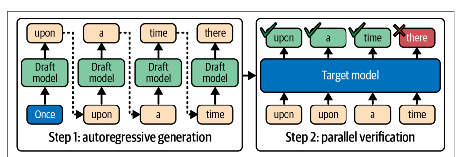
Once the target model’s corrected token is used and decoding continues, a new speculative decoding cycle can start from that point. Figure 15-8 shows a small draft model predicting multiple tokens ahead. Then the target (big) model verifies these tokens one by one.一旦使用了目标模型修正后的 token 并继续解码，就可以从该点开始新一轮投机解码循环。图 15-8 展示了一个小型草稿模型向前预测多个 token，随后目标（大）模型逐个验证这些 token。

Over time, speculative decoding reduces the overall number of one-by-one, sequential invocations needed by the large model. In theory, it provides a theoretical k× speedup, where k is the number of tokens generated by the draft model. In practice, with overhead and occasional speculative-token rejections, the gain is more like a 2× speedup.随着时间推移，投机解码减少了大模型所需的逐个、串行调用的总次数。理论上，它可提供 k× 的加速，其中 k 是草稿模型生成的 token 数。在实践中，考虑到额外开销和偶发的投机 token 被拒绝，收益更接近 2× 加速。

The draft model must be chosen to have reasonably high fidelity to the large model’s distribution. This means that the draft model’s predictions should have high overlap with the large model’s likely outputs. If the draft frequently guesses wrong, speculative decoding provides little benefit and wastes compute. If it often predicts tokens that the larger target model would not, many speculative tokens will be rejected. This will waste compute time.必须选择与大模型分布具有相当高保真度的草稿模型。这意味着草稿模型的预测应与大模型可能的输出高度重叠。如果草稿模型经常猜错，投机解码带来的收益很小，还会浪费算力。如果它经常预测出更大的目标模型不会产生的 token，那么许多投机 token 将被拒绝，这会浪费计算时间。

The draft model must also be much faster than the large model—typically by a factor of 4× or more—for speculative decoding to provide a practical performance improvement. A common strategy is to use a distilled version of the main model—or a smaller model fine-tuned on the same data so that its outputs correlate well.草稿模型还必须比大模型快得多——通常快 4× 或以上——投机解码才能带来实际的性能提升。一种常见策略是使用主模型的蒸馏版本，或使用在同一数据上微调过的更小模型，使其输出具有良好相关性。

The draft model generates tokens using the same prompt and perhaps a higher temperature to increase the chance of matching one of the large model’s probable continuations. Meanwhile, the target model skips ahead and processes all of the draft tokens in one single batch.草稿模型使用相同的提示词生成 token，并且可能采用更高的温度（temperature），以提高命中大模型某个可能续写结果的机会。与此同时，目标模型向前跳跃，在单个批次中处理全部草稿 token。

Under the standard speculative decoding acceptance procedure, the target model’s output distribution is preserved. As such, the final samples match the large model’s distribution when sampling settings are aligned. If the draft diverges, the target model’s verification rejects those tokens and correctness is maintained. The only difference is that up to k number of target-model calls are avoided when the small model guesses correctly for these speculative tokens.在标准的投机解码接受流程下，目标模型的输出分布得以保持。因此，当采样设置对齐时，最终采样结果与大模型的分布一致。如果草稿出现分歧，目标模型的验证会拒绝这些 token，正确性得以维持。唯一的区别在于，当小模型对这些投机 token 猜测正确时，最多可避免 k 次目标模型调用。

Speculative decoding can be implemented in a variety of ways. Most modern LLM inference engines like vLLM, SGLang, and TensorRT-LLM have built-in support to coordinate draft and target model generation. Empirically, speedups around 1.5–2.5× are common, and higher gains are possible with careful batching and draft model design.投机解码（speculative decoding）可以通过多种方式实现。vLLM、SGLang 和 TensorRT-LLM 等大多数现代 LLM 推理引擎都内置支持协调草稿模型与目标模型的生成。根据经验，1.5–2.5× 左右的加速很常见，而通过精心的批处理与草稿模型设计，还可能获得更高收益。

For instance, the Extrapolation Algorithm for Greater LLM Efficiency (EAGLE) algorithm rethinks speculative decoding by operating at the feature level rather than the token level. EAGLE uses a one-step extrapolation of the large model’s own intermediate representation to predict the next token’s features. This resolves uncertainty and achieves higher acceptance rates.例如，更大 LLM 效率的外推算法（Extrapolation Algorithm for Greater LLM Efficiency，EAGLE）重新思考了投机解码，它在特征层面而非词元层面运作。EAGLE 利用大模型自身中间表示的一步外推来预测下一个词元的特征。这消除了不确定性，并实现了更高的接受率。

EAGLE reported up to about 3.5× speedup over vanilla decoding for a 4-token draft while preserving the large model’s output distribution. EAGLE approaches the theoretical limit of its draft depth in favorable environments. And it shows that, with innovative techniques, speculative decoding can reduce decoding time even further— and preserve output quality at the same time.EAGLE 报告称，在 4 词元草稿下，相比原始解码最高可获得约 3.5× 的加速，同时保持大模型的输出分布。在有利环境中，EAGLE 已接近其草稿深度的理论上限。并且它表明，借助创新技术，投机解码可以进一步缩短解码时间——同时保持输出质量。

EAGLE-2 extends EAGLE by introducing a context-aware dynamic draft tree of possibilities. While EAGLE achieved up to 3.5× speedup versus vanilla decoding in some evaluations, EAGLE-2’s approach reported speedups of about 20%–40% faster than EAGLE depending on the task and model. With EAGLE-2, the draft model generates a branching set of token sequences, which further increases parallelism in the verification step. This is shown in Figure 15-9.EAGLE-2 通过引入上下文感知的动态*草稿树*来扩展 EAGLE。尽管在某些评估中 EAGLE 相比原始解码最高实现了 3.5× 加速，但 EAGLE-2 的方法报告称，根据任务和模型的不同，其速度比 EAGLE 快约 20%–40%。借助 EAGLE-2，草稿模型会生成一组分支化的词元序列，这进一步提升了验证步骤中的并行度。如图 15-9 所示。

EAGLE-3 continues to improve on earlier versions, EAGLE-1 and EAGLE-2, by preferring direct token prediction and fusing multi-layer features. EAGLE-3 reports up to 1.4× improvements over EAGLE-2 in certain tasks—and up to 6.5× speedups over non-optimized baseline variants. In EAGLE-1 and EAGLE-2, the draft model predicts internal feature vectors which are then decoded to tokens. These earlier EAGLE methods worked by guessing internal features, essentially—and then mapping them to tokens.EAGLE-3 通过倾向于直接预测词元并融合多层特征，持续改进早期版本 EAGLE-1 和 EAGLE-2。EAGLE-3 报告称，在某些任务上相比 EAGLE-2 最高提升 1.4×——相比未优化的基线变体最高加速 6.5×。在 EAGLE-1 和 EAGLE-2 中，草稿模型预测内部特征向量，然后再解码为词元。这些早期 EAGLE 方法本质上是通过猜测内部特征、再将其映射为词元来工作的。

EAGLE-3 skips the feature-level prediction step and predicts the draft tokens more directly. However, it still uses internal features but fused into multiple layer representations (lower, middle, upper) to guide the draft predictions. This is in contrast to using just the top layer. This makes EAGLE-3 more streamlined and less constrained—allowing better scaling.EAGLE-3 跳过了特征层面的预测步骤，更直接地预测草稿词元。不过，它仍然使用内部特征，但将其融合为多层表示（低层、中层、高层）来引导草稿预测。这与仅使用顶层形成对比。这使得 EAGLE-3 更精简、约束更少——从而实现更好的扩展。

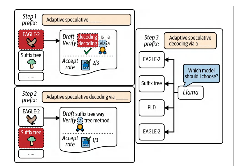
Another technique is dynamic depth decoding, which can adaptively skip layers that minimize the impact on output quality. Other techniques that reduce computations include skipping every *N*th transformer layer, using lower precision (e.g., FFP8 and NVFP4) for the draft model, and using a smaller hidden size temporarily for the draft stage.另一项技术是*动态深度解码*，它可以自适应地跳过对输出质量影响最小的层。其他减少计算的技术包括：跳过每第 N 个 Transformer 层、为草稿模型使用更低精度（例如 FFP8 和 NVFP4），以及在草稿阶段临时使用更小的隐藏维度。

Future LLMs might include an optimized “fast-generation” mode. For example, a model might have alternate lightweight layers or a configuration for reduced-precision decoding. This built-in optimization would allow the model to skip computations.未来的 LLM 可能会包含优化的“快速生成”模式。例如，模型可能具有交替的轻量层，或用于降低精度解码的配置。这种内置优化将允许模型跳过计算。

单模型自投机解码

Single-Model Self-Speculative Decoding

Another approach to speculative decoding is to avoid using an external draft model altogether and use the larger target model to both draft and verify its own outputs by selectively skipping some computations. One such method is self-speculative decoding, also called the draft-and-verify scheme.投机解码（speculative decoding）的另一条思路是完全不使用外部草稿模型，而是让更大的目标模型通过有选择地跳过部分计算，自行完成草稿生成与输出验证。其中一种方法称为自投机解码（self-speculative decoding），也称为草稿-验证方案（draft-and-verify）。

With self-speculative decoding, the large target model generates k tokens using a fast, approximate pass. For instance, it can choose to run only half of its layers—and possibly in reduced precision—for each new token. It would skip every other layer. This produces draft output much like the smaller draft model would. And it can approach similar speedups when acceptance rates and draft depth are favorable. This produces draft output much like the smaller draft model would—and achieves a similar 2× speedup as well.在自投机解码中，大型目标模型通过一次快速近似前向过程生成 k 个 token。例如，它可以为每个新 token 只运行一半的层——并且可能使用更低的精度。它会跳过每隔一层的层。这样产生的草稿输出与较小的草稿模型所产生的非常相似。并且在接受率和草稿深度有利时，它可以接近类似的加速比。这样产生的草稿输出与较小的草稿模型所产生的非常相似——并且同样能实现约 2× 的加速。

Then, in a second stage of self-speculative decoding, the target model performs a full forward pass to verify those k tokens in one go. If they all match, then we save executing half the layers for those tokens. If not, we simply fall back to the traditional speculative approach by accepting tokens up to the mismatch and proceeding normally.随后，在自投机解码的第二阶段，目标模型执行一次完整的前向传播，一次性验证这 k 个 token。如果它们全部匹配，我们就为这些 token 省去了执行一半的层。如果不匹配，我们只需回退到传统的投机方法：接受到不匹配处为止的 token，然后正常继续。

Because it’s the same model doing both draft and verification in self-speculative decoding, no separate model needs to be trained, maintained, or loaded into memory at runtime. The challenge is finding a good way to reduce the amount of compute needed in the draft stage (dropping layers, reducing precision, etc.) without hurting accuracy too much.由于在自投机解码中由同一个模型同时完成草稿生成与验证，因此无需训练、维护或在运行时将单独的模型加载到内存中。难点在于找到一种好方法，在不显著损害精度的前提下减少草稿阶段所需的计算量（丢弃层、降低精度等）。

A related technique is consistent decoding, in which you train one LLM to both generate and validate multiple tokens. This single-model approach produces ~3× speedups without a separate draft model. This shows a trend of baking speculative decoding into the model’s own weights.一项相关技术是*一致性解码*（consistent decoding），即训练单个 LLM 同时生成并验证多个 token。这种单模型方法无需单独的草稿模型即可带来约 3× 的加速。这体现出一种将投机解码固化到模型自身权重中的趋势。

These methods represent very active areas of research. And they are particularly exciting and promising because they let the model accelerate itself using its inherent internal redundancy. And since the optimizations are local to the model, the inference engine’s implementation can be simplified.这些方法属于非常活跃的研究领域。它们尤其令人兴奋且前景广阔，因为它们让模型利用自身固有的内部冗余来加速自己。并且由于这些优化局限于模型内部，推理引擎的实现也可以得到简化。

使用 Medusa 多头的多 token 解码

Multitoken Decoding with Medusa’s Multiple Heads

Speculative decoding still ultimately generates tokens one by one using the draft model—it’s just faster because the draft model is smaller. However, the Medusa framework takes a more radical approach. It modifies the model architecture itself to predict multiple new tokens in parallel for each decoding step.投机解码最终仍然要借助草稿模型逐个生成 token——只是由于草稿模型更小所以更快。然而，Medusa 框架采取了更为激进的做法。它修改模型架构本身，使每个解码步骤能够并行预测多个新 token。

Unlike two-model speculative decoding, which still generates tokens one by one (albeit faster), Medusa’s architecture truly generates multiple tokens per iteration from a single model. As such, Medusa’s multiheaded approach has reported about 2.2–3.6× speedups in published experiments across both Medusa-1 and Medusa-2.双模型投机解码仍然逐个生成 token（尽管更快），与之不同，Medusa 的架构真正从单个模型在每次迭代中生成多个 token。因此，据已发表的实验报告，Medusa 的多头方法在 Medusa-1 和 Medusa-2 上均实现了约 2.2–3.6× 的加速。

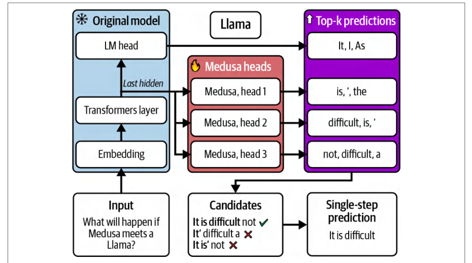
However, Medusa requires custom model training since it modifies the transformer-based LLM with additional decoder heads that branch off at certain layers—hence, the name Medusa. This lets the model propose several next tokens simultaneously.然而，Medusa 需要定制化的模型训练，因为它为基于 Transformer 的 LLM 增加了额外的解码头，这些解码头在某些层处分叉出来——Medusa（美杜莎）之名正源于此。这使得模型能够同时提出若干个后续 token。

The multiple token candidates generated by the different Medusa heads are structured like a tree. For instance, Medusa can generate a binary tree of depth 2 in one pass to produce up to 4 tokens. It can then verify the sequence of multiple tokens in parallel, as shown in Figure 15-10.不同 Medusa 头生成的多个候选 token 以树状结构组织。例如，Medusa 可以在一次前向中生成深度为 2 的二叉树，从而产生最多 4 个 token。随后它可以并行验证这多个 token 组成的序列，如图 15-10 所示。

Internally, Medusa uses a specialized, tree-based attention pattern to improve consistency among the parallel token predictions. The model learns to extend and verify the multiple-token sequences concurrently. With Medusa, the LLM essentially learns to “think ahead” by a few tokens—and output them all at once.在内部，Medusa 使用专门的树状注意力模式，以提高并行 token 预测之间的一致性。模型学会并发地扩展并验证多 token 序列。借助 Medusa，LLM 实质上学会了“提前思考”若干个 token——并一次性将它们全部输出。

During inference, Medusa can reduce the number of sequential decoding iterations by the factor of the parallel predictions. For instance, if Medusa predicts 4 tokens in one pass, it can reduce the required number of forward passes by up to 4× for depth-2 binary tree outputs.在推理过程中，Medusa 可以按并行预测的倍数减少串行解码迭代的次数。例如，如果 Medusa 在一次前向中预测 4 个 token，那么对于深度为 2 的二叉树输出，它可以将所需的前向传播次数最多减少 4 倍。

In practice, however, Medusa typically achieves about a 2–3× speedup due to the overhead of occasionally having to backtrack when a prediction branch fails validation and needs a partial redo. This is similar to the overhead of speculative decoding verification and rejection. For example, if a Medusa LLM generates 4 tokens per iteration, a reply of 100 tokens would take only 25 iterations of the model instead of 100.然而在实践中，Medusa 通常只能实现约 2–3 倍的加速，因为当某个预测分支未通过验证、需要部分重做时，偶尔必须回退，这会带来额外开销。这与投机解码（speculative decoding）的验证与拒绝开销类似。例如，如果一个 Medusa LLM 每次迭代生成 4 个 token，那么 100 个 token 的回复只需模型迭代 25 次，而不是 100 次。

Medusa requires modifying and retraining the model to add these extra heads. In addition, Medusa models are slightly larger in size given the additional head parameters. This increases development complexity and training cost a bit. However, once trained, Medusa models can significantly reduce inference times.Medusa 需要修改并重新训练模型以添加这些额外的头。此外，由于增加了头参数，Medusa 模型的体积会略大一些。这在一定程度上增加了开发复杂度和训练成本。然而，一旦训练完成，Medusa 模型可以显著缩短推理时间。

If trained for your use case, a Medusa-enabled LLM can provide excellent low-latency performance. However, this technique requires modifying and fine-tuning the model architecture to add the additional heads.如果针对你的用例进行训练，启用 Medusa 的 LLM 可以提供出色的低时延性能。然而，该技术需要修改并微调模型架构以添加额外的头。

交错执行多个请求的解码步骤

Interleaving Decode Steps from Multiple Requests

Another parallel decoding technique is to interleave decode steps from multiple concurrent requests across multiple end users. This parallelism is more of an inference-engine capability than an algorithmic trick or model architecture modification. But it helps keep the GPUs busy by batching at the token level—and across end-user requests.另一种并行解码技术是交错执行来自多个终端用户的多个并发请求的解码步骤。这种并行性更多是推理引擎的一项能力，而非算法技巧或模型架构修改。但它通过在 token 级别进行批处理——并且跨终端用户请求进行批处理——帮助让 GPU 保持忙碌。

Frameworks like vLLM implement this in the form of request routing, continuous batching, and token scheduling. The idea is to keep the GPUs busy by filling in the gaps between sequential steps. Specifically, if a GPU is stalled due to a sequence waiting on I/O or a data dependency, the scheduler can run another sequence’s next token prediction on that same GPU in the meantime.vLLM 等框架以请求路由、连续批处理（continuous batching）和 token 调度的形式实现了这一点。其思路是通过填补串行步骤之间的空隙来让 GPU 保持忙碌。具体来说，如果某个 GPU 因某个序列在等待 I/O 或数据依赖而停滞，调度器可以在此期间在同一 GPU 上运行另一个序列的下一个 token 预测。

It’s important to note that interleaving decode steps doesn’t speed up a single sequence’s latency. In fact, it can even add a tiny bit of overhead per token due to the additional context switching. However, it can greatly improve overall throughput and GPU utilization when serving many users concurrently. This will reduce the average end-user request latency under heavy load.需要注意的是，交错执行解码步骤并不会加快单个序列的时延。事实上，由于额外的上下文切换，它甚至可能为每个 token 增加一点点开销。然而，在同时服务大量用户时，它可以大幅提升整体吞吐量和 GPU 利用率。这会降低高负载下的平均终端用户请求时延。

组合使用解码技术并评估复杂度

Combining Decoding Techniques and Evaluating Complexity

It’s worth noting that these decoding optimizations can be combined. For instance, one could use speculative decoding with a Medusa-enabled target model in which the big target model verifies multiple tokens at a time predicted by a small model.值得注意的是，这些解码优化可以组合使用。例如，可以将投机解码与启用 Medusa 的目标模型结合使用，由大的目标模型一次性验证小模型预测的多个 token。

These techniques also come at the cost of additional complexity. Either you have to maintain an extra model, alter the main model, or manage more elaborate control logic. In production, you should evaluate this complexity against the performance gains. For interactive applications, reducing response time by even a few milliseconds is worth the complexity—especially at scale.这些技术也以额外的复杂度为代价。你要么必须维护一个额外的模型，要么必须改动主模型，要么必须管理更复杂的控制逻辑。在生产环境中，你应当权衡这种复杂度与性能收益。对于交互式应用，即使只把响应时间缩短几毫秒，也值得为此付出复杂度——尤其是在大规模场景下。

In short, advanced decoding techniques like speculative decoding—with or without a draft model—and Medusa-style multitoken prediction can reduce overall inference times of modern autoregressive LLMs that traditionally generate one token at a time. By generating more tokens at a time, increasing overall arithmetic intensity, and pushing the decoding step toward the compute-bound regime, you can take advantage of the GPU’s extreme compute capabilities.简而言之，诸如推测解码（无论是否使用草稿模型）以及 Medusa 风格的多 token 预测等高级解码技术，能够缩短现代自回归 LLM 的整体推理时间——这类模型传统上每次只生成一个 token。通过一次生成更多 token、提高整体算术强度，并推动解码步骤向计算受限区间靠拢，你就可以充分利用 GPU 极强的计算能力。

约束解码的性能影响

Constrained Decoding Performance Implications

A separate but important aspect of the LLM decoding process is generating text under certain constraints. For instance, the model can force the output to match a predefined format (JSON), use a particular grammar, or disallow certain sequences for safety. As such, constrained decoding, often called structured outputs, is often required for production use cases.LLM 解码过程中另一个独立但重要的方面是：在特定约束下生成文本。例如，模型可以强制输出匹配预定义格式（JSON）、使用特定语法，或出于安全考虑禁止某些序列。因此，约束解码（常被称为*结构化输出*）在生产用例中往往是必需的。

OpenAI’s function-calling API, for example, relies on well-structured output formats to determine which function to call—as well as the functions’ inputs and outputs. These constraints are designed to match the function’s API signature and are simply nonnegotiable at the application level.例如，OpenAI 的函数调用 API 依赖结构良好的输出格式来确定调用哪个函数，以及函数的输入与输出。这些约束被设计为与函数的 API 签名相匹配，在应用层面毫无商量余地。

Constrained decoding alters the model’s token-selection process so that, at each step, only valid tokens are allowed. This might be as simple as supplying a list of allowed tokens—or as sophisticated as embedding a formal grammar and using a state machine to filter out invalid tokens.约束解码会改变模型的 token 选择过程，使得每一步只允许出现合法的 token。这可以简单到提供一份允许的 token 列表，也可以复杂到嵌入形式化语法并用状态机过滤掉非法 token。

The drawback of constrained decoding is that extra latency is needed to enforce these constraints—often a few milliseconds per token. This is because the model may need to backtrack repeatedly, navigate the pruned vocabulary, and ultimately generate a valid token. Backtracking happens inside the LLM’s generation loop. As such, debugging, profiling, and tuning constrained decoding can be difficult without fine-grained telemetry in the model itself.约束解码的缺点在于：执行这些约束会带来额外时延——通常为每个 token 几毫秒。这是因为模型可能需要反复回溯、在剪枝后的词表中导航，最终才生成一个合法 token。回溯发生在 LLM 的生成循环内部。因此，若模型本身缺乏细粒度遥测，调试、性能剖析和调优约束解码都会很困难。

Another performance consideration is cache efficiency. Pruning the full probability distribution at every decode step can blow caches and reduce throughput even further. This is particularly noticeable when the allowed token set is heavily limited.另一个性能考量是缓存效率。在每个解码步骤对完整概率分布进行剪枝，可能会冲垮缓存，进一步降低吞吐量。当允许的 token 集合受到严格限制时，这一点尤为明显。

To mitigate these costs, many frameworks compile a JSON grammar and precompute valid tokens for each state. This allows the inference engine to mask out invalid softmax outputs at runtime. This approach reduces backtracking, improves caching, and raises acceptance rates.为缓解这些开销，许多框架会编译 JSON 语法，并为每个状态预先计算合法 token。这样推理引擎就能在运行时屏蔽掉非法的 softmax 输出。该方法减少了回溯、改善了缓存，并提高了接受率。

For moderate constraints such as simple JSON schemas, modern engines that use compiled grammars and overlap mask computation with GPU execution can push overhead into the low single-digit percent range at scale, but complex grammars or small batches can still incur double-digit overhead. Always measure TTFT and tokens per second under your exact schema.对于简单 JSON schema 这类中等程度的约束，采用编译语法并将掩码计算与 GPU 执行重叠的现代引擎，在大规模下可将开销压到较低的个位数百分比区间；但复杂语法或小批大小仍可能带来两位数的开销。请务必在你实际使用的 schema 下测量 TTFT 和每秒 token 数。

These techniques have been implemented in popular libraries and inference engines, including Hugging Face Transformers, NVIDIA NeMo, and vLLM. For instance, NVIDIA’s TensorRT-LLM and Hugging Face Transformers both allow user-defined vocabulary masks to enforce constraints with negligible speed penalty. Specifically, TensorRT-LLM exposes guided decoding with JSON schema and context-free grammar (CFG) support through the XGrammar backend. And vLLM and Transformers provide structured output APIs.这些技术已在主流库和推理引擎中实现，包括 Hugging Face Transformers、NVIDIA NeMo 和 vLLM。例如，NVIDIA 的 TensorRT-LLM 和 Hugging Face Transformers 都允许用户自定义词表掩码来施加约束，而速度损失可以忽略不计。具体而言，TensorRT-LLM 通过 XGrammar 后端提供支持 JSON schema 和上下文无关语法（CFG）的引导式解码。vLLM 和 Transformers 则提供结构化输出 API。

Another popular strategy is to push constrained decoding into the kernel itself. In this case, it would inject token masks during the final softmax step to achieve similar performance gains.另一种常见策略是把约束解码下推到内核本身。在这种情况下，它会在最后的 softmax 步骤中注入 token 掩码，以获得类似的性能收益。

When implemented efficiently, constrained decoding can often run as fast as unconstrained decoding—especially if the constraint ruleset is not too large or too restrictive. If the decoding constraints are too restrictive, decoding effectively becomes a search through a small token space. This leads to more backtracking and slower token generation.如果实现得当，约束解码的运行速度往往与无约束解码相当——尤其是当约束规则集不太大、限制也不太严格时。如果解码约束过于严格，解码实际上就变成了在很小的 token 空间中进行搜索。这会导致更多回溯，token 生成变慢。

MoE 推理的动态路由策略

Dynamic Routing Strategies for MoE Inference

Serving MoE models efficiently requires careful partitioning of experts across GPUs using expert parallelism. In addition, you need an intelligent and dynamic mechanism, or gating network, to dynamically route tokens to these experts at runtime.高效地服务 MoE 模型，需要用专家并行把专家谨慎地划分到各块 GPU 上。此外，还需要一个智能的动态机制，即门控网络，在运行时把 token 动态路由到这些专家。

During MoE inference, each token’s forward pass must be routed by the gating network to one or more expert GPUs. The system needs to handle this communication in a balanced way to keep the GPUs busy—and avoid overloaded GPUs, or hotspots. Let’s examine how to address these in a high-scale, multinode inference environment.在 MoE 推理过程中，每个 token 的前向传播都必须由门控网络路由到一块或多块专家 GPU。系统需要以均衡的方式处理这种通信，让 GPU 保持忙碌——并避免 GPU 过载或出现热点。下面我们来看看在高规模、多节点推理环境中如何解决这些问题。

专家通信优化

Expert Communication Optimization

During the all-to-all exchange of token activations across experts, an MoE shuffles a batch of tokens between the GPUs. Each GPU receives only the tokens it needs for the experts that it hosts, as shown in Figure 15-11. This happens for every layer in the MoE and is a costly operation, which can potentially dominate inference time if not handled efficiently.在跨专家交换 token 激活值的全对全（all-to-all）过程中，MoE 会在各块 GPU 之间打乱一批 token。每块 GPU 只接收其托管的专家所需的 token，如图 15-11 所示。MoE 的每一层都会发生这一过程，这是一项开销很大的操作，如果处理不当，可能会主导推理时间。

One strategy to reduce communication overhead is to use a hierarchical routing strategy for our GPU cluster by first routing tokens between GPUs within the same node using NVSwitch/NVLink (fast) and routing across nodes only for any remaining tokens that need nonlocal experts. This two-stage all-to-all can reduce the volume of internode traffic.降低通信开销的一种策略是为 GPU 集群采用分层路由策略：先使用 NVSwitch/NVLink 在同一节点内的 GPU 之间路由 token（速度快），只对需要非本地专家的剩余 token 进行跨节点路由。这种两阶段全对全可以减少节点间流量。

Additionally, you can use asynchronous communication by overlapping the communication with computation. High-performance MoE inference servers use double-buffer communications so that while one batch of tokens is being sent around, the previous batch’s expert computations occur in parallel. This pipelining hides much of the communication latency.此外，还可以通过将通信与计算重叠来实现异步通信。高性能 MoE 推理服务器使用双缓冲通信，使得在一批 token 被发送的同时，上一批 token 的专家计算并行进行。这种流水线化隐藏了大部分通信时延。

A naive implementation of expert routing that uses a single global all-to-all barrier can leave GPUs waiting on synchronization overhead. This wastes bandwidth if not all links are utilized optimally.如果专家路由的朴素实现使用单一的全局全对全屏障，就会让 GPU 因同步开销而等待。如果并非所有链路都被最优利用，这还会浪费带宽。

Techniques such as a butterfly schedule (aka shifted all-to-all schedule) can break the communication into phased rounds. This way, every NVLink/NIC is busy with partial exchanges—as opposed to one big synchronization. This staggered approach improves link utilization and reduces idle time.诸如*蝶形调度*（又称*移位全对全（all-to-all）调度*）之类的技术可以将通信拆分为多个分阶段的轮次。这样一来，每个 NVLink/NIC 都忙于部分交换——而不是进行一次大规模同步。这种交错方式提升了链路利用率并减少了空闲时间。

All-to-all exchanges may use the built-in ncclAllToAll collective or grouped send and receive calls. Throughput often improves when the exchange is chunked and pipelined or when a hierarchical schedule such as butterfly is used across nodes. Validate and choose the algorithm that matches your topology.全对全交换可以使用内置的 ncclAllToAll 集合通信操作，或分组的发送与接收调用。当交换被分块并流水线化，或在跨节点时采用蝶形等分层调度时，吞吐量通常会有提升。请验证并选择与你的拓扑相匹配的算法。

Another solution to reduce communication traffic is called *expert collocation. *The idea is to collocate certain experts together on the same GPU or node to avoid unnecessary communication. Consider two experts, experts 5 and 7, that are often activated for the same token by the token router. Placing experts 5 and 7 on the same GPU can eliminate an extra all-to-all hop. Profiling tools and gating-frequency analysis can help identify such pairings for your workload.另一种减少通信流量的方案称为*专家并置（expert collocation）*。其思路是将某些专家并置在同一块 GPU 或同一个节点上，以避免不必要的通信。设想专家 5 和专家 7 这两个专家经常被 token 路由器针对同一个 token 激活。将专家 5 和 7 放在同一块 GPU 上可以消除一次额外的全对全跳。性能剖析工具与门控频率分析可以帮助你为自身工作负载识别出这类配对。

And yet another solution is to compress the communication between experts, including expert-exchange activations. For instance, you can cast to FP8 or NVFP4 on Tensor Cores with the NVIDIA Transformer Engine before performing an all-to-all communication. This will reduce NIC load which amortizes the compression computation. This trades a tiny bit of numerical precision for faster activation transfers between GPUs. The overhead to cast and pack/unpack is usually small relative to network and memory transfer costs.还有一种方案是压缩专家之间的通信，包括专家交换的激活值。例如，你可以在执行全对全通信之前，使用 NVIDIA Transformer Engine 在张量核心上转换为 FP8 或 NVFP4。这会降低 NIC 负载，从而摊薄压缩计算的开销。这以极小的数值精度损失换取 GPU 之间更快的激活值传输。相对于网络与内存传输开销，转换以及打包/解包的开销通常很小。

In short, optimizing MoE communication involves analyzing the hardware and network topology to optimize the placement of experts onto GPUs. For your deployments, it’s important to configure the cluster’s interconnects for efficient all-to-all communication. For instance, use the NVLink Switch mesh in an NVL72 rack to get the full bandwidth communication between up to 72 GPUs in a single domain. Naive all-to-all choices can dominate layer time and achieve very low SM efficiency. Prioritize expert traffic and overlap where possible, and make sure to profile and verify when making different interconnect and communication-algorithm choices.简而言之，优化 MoE 通信需要分析硬件与网络拓扑，以优化专家在 GPU 上的放置。对于你的部署而言，重要的是配置集群的互连，以实现高效的全对全通信。例如，在 NVL72 机架中使用 NVLink Switch 网格，即可在单一域内最多 72 块 GPU 之间获得全带宽通信。朴素的全对全选择可能主导层耗时，并导致极低的 SM 效率。优先处理专家流量并尽可能重叠，同时在做出不同的互连与通信算法选择时，务必进行剖析与验证。

负载均衡、容量因子与专家复制

Load Balancing, Capacity Factor, and Expert Replication

It’s recommended that each expert and GPU get an equal share of the work to avoid “hotspots.” Otherwise, if the MoE’s gating network directs a disproportionate number of tokens to a particular expert, those GPUs will become overloaded. This will increase latency and reduce overall system throughput.建议让每个专家和每块 GPU 获得均等的工作份额，以避免“热点”。否则，如果 MoE 的门控网络将不成比例的 token 导向某个特定专家，那些 GPU 就会过载。这会增加时延并降低整体系统吞吐量。

Consider a single expert GPU that becomes a hotspot with utilization hitting 99% while the other expert GPUs are averaging around 60% utilization. This can bottleneck an entire training or inference cluster if not properly handled.设想某一块专家 GPU 成为热点，利用率达到 99%，而其他专家 GPU 的平均利用率约为 60%。如果处理不当，这会使整个训练或推理集群出现瓶颈。

During model training, hotspots can be addressed by adding a load-balancing loss term that penalizes the gate if it overuses some experts and underuses others. The result is that the trained MoE model tends to distribute tokens fairly evenly across the experts.在模型训练期间，可以通过增加一个负载均衡损失项来解决热点问题，该项会在门控过度使用某些专家而使用不足其他专家时对其进行惩罚。其结果是，训练得到的 MoE 模型倾向于将 token 较为均匀地分配到各个专家上。

At inference time, however, specific input prompts or topics might still cause imbalance by concentrating on a subset of “hot” experts. One strategy to avoid inference hot spots is to use a capacity factor that triggers an overflow mechanism.然而在推理时，特定的输入提示或主题仍可能集中在少数“热点”专家上，从而造成不均衡。避免推理热点的一种策略是使用*容量因子*（capacity factor）来触发溢出机制。

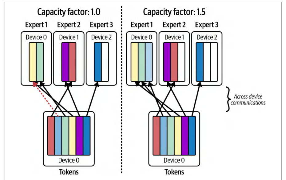
By specifying a capacity factor, the model can be configured such that each expert can process only a maximum number of tokens (e.g., 32 tokens) at a given time. If an expert receives more than this capacity of tokens, the extra tokens can either be for-warded to a fallback expert with the next highest routing score or the tokens will be serialized and processed in a second pass. Figure 15-12 compares a capacity factor of 1.0 versus 1.5.通过指定容量因子，可以将模型配置为每个专家在给定时间内最多只处理一定数量的 token（例如 32 个 token）。如果某个专家收到的 token 超过该容量，多出的 token 既可以转发给路由分数次高的后备专家，也可以被串行化并在第二轮中处理。图 15-12 对比了容量因子 1.0 与 1.5 的情况。

In practice, a capacity factor of 1.2 (20% overflow allowance) with top-2 gating is common. This means that each expert will take up to 120% of its average load. After that, it will send excess tokens to the next expert. This will effectively smooth out the load across experts in the system.在实践中，配合 top-2 门控使用 1.2 的容量因子（允许 20% 溢出）很常见。这意味着每个专家最多承担其平均负载的 120%。超过之后，它会把多余的 token 发送给下一个专家。这能有效平滑系统中各专家之间的负载。

Another strategy to avoid hotspots is expert replication. If one expert is consistently a hotspot, the system can clone that expert onto another GPU. This way, the gating function can send some fraction of tokens to the expert clone running on the other GPU.另一种避免热点的策略是专家复制（expert replication）。如果某个专家持续成为热点，系统可以将该专家克隆到另一块 GPU 上。这样，门控函数就可以把一部分 token 发送给运行在另一块 GPU 上的专家副本。

The replicas are a pure application-level optimization implemented by the inference engine. The model itself is not aware of the replicas. Because replicas are registered as separate experts with their own indices—and often on different GPUs—the engine can route tokens across both the original experts and their clones according to their relative routing scores.副本纯粹是由推理引擎实现的应用层优化。模型本身并不知道副本的存在。由于副本被注册为具有各自索引的独立专家——而且通常位于不同的 GPU 上——引擎可以根据相对路由分数，在原始专家及其克隆之间路由 token。

Also, replication requires careful handling to keep the replicas synchronized if the model is updated. It’s important that all replica experts remain identical (e.g., same weights) since the gating router knows about only a single expert and does not actually know about the replicas.此外，如果模型发生更新，复制还需要谨慎处理以保持副本同步。所有副本专家必须保持一致（例如相同的权重），这一点很重要，因为门控路由器只知道单个专家，实际上并不知道副本的存在。

自适应专家路由与实时监控

Adaptive Expert Routing and Real-Time Monitoring

Unlike traditional MoE expert gating, which is fixed after training, adaptive routing can adjust the gate’s decisions in real time during inference to react to current conditions and expert load. For instance, if the system detects that one expert GPU is lagging behind, it could instruct the gating function to divert some tokens to another expert. The other expert might have a slightly lower routing score, but it receives the request because it has available capacity.与训练后即固定的传统 MoE 专家门控不同，自适应路由可以在推理期间实时调整门控的决策，以响应当前状况和专家负载。例如，如果系统检测到某块专家 GPU 落后，它可以指示门控函数将部分 token 转移到另一个专家。另一个专家的路由分数可能略低，但由于它还有可用容量，因此会接收该请求。

You should implement continuous monitoring of per-expert utilization and response latency metrics. Modern MoE systems integrate with telemetry frameworks such that each expert emits utilization metrics to Prometheus/Grafana. This way, the system can dynamically adjust the capacity factor or gating algorithm on the fly.应当对每个专家的利用率和响应时延指标实施持续监控。现代 MoE 系统会与遥测框架集成，使每个专家向 Prometheus/Grafana 上报利用率指标。这样，系统就能动态地即时调整容量因子或门控算法。

Most LLM expert gating functions only consider routing scores determined at training time. However, a truly adaptive system needs to be handled by the inference engine and performed dynamically at inference time.大多数 LLM 专家门控函数只考虑训练时确定的路由分数。然而，真正自适应的系统需要由推理引擎处理，并在推理时动态执行。

To implement adaptive routing, the inference engine needs to wrap the model’s forward pass in custom logic. For example, it can intercept the gating softmax and reallocate some tokens to different experts based on current load metrics.要实现自适应路由，推理引擎需要把模型的前向传播包裹在自定义逻辑中。例如，它可以拦截门控 softmax，并根据当前负载指标把部分 token 重新分配给不同的专家。

Inference engines rely on real-time metrics like per-GPU utilization and per-expert token counts to continuously measure expert load. If the system sees one expert’s GPU at 99% utilization while other experts’ GPUs are at 60%, the system could temporarily lower its load by routing some tokens to its expert replica—or to a different expert with a slightly lower expert-preference score.推理引擎依赖每 GPU 利用率和每专家 token 数等实时指标来持续测量专家负载。如果系统发现某个专家的 GPU 利用率达到 99%，而其他专家的 GPU 为 60%，系统就可以临时降低其负载，把部分 token 路由到该专家的副本——或路由到专家偏好分数略低的其他专家。

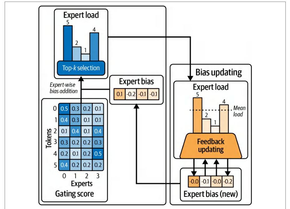
Figure 15-13 shows an adaptive MoE routing strategy that uses a biased gating score approach. While this approach was originally used in a training context, a simpler approach applies to inference. In this case, it would use a modified expert-bias algorithm to divert tokens to alternate experts when the primary experts are heavily loaded.图 15-13 展示了一种采用偏置门控分数方法的自适应 MoE 路由策略。虽然该方法最初用于训练场景，但有一种更简单的方法适用于推理。在这种情况下，它会使用改进的专家偏置算法，在主专家负载很重时把 token 转移到备选专家。

This approach can reduce unnecessary communication and balance the load more uniformly. However, it does incur some additional cost in the form of extra monitoring, decision making, complexity, configuration management, and logging. The benefits may or may not outweigh the cost. Every scenario and workload is unique, but it’s definitely something worth exploring.这种方法可以减少不必要的通信，并更均匀地平衡负载。然而，它确实会带来一些额外成本，表现为额外的监控、决策、复杂性、配置管理和日志记录。收益是否超过成本并不确定。每个场景和工作负载都是独特的，但这绝对值得探索。

When profiling with tools like Nsight Systems, you want to monitor the timeline traces of the expert GPUs’ all-to-all communications. If one GPU’s segment in the timeline is much longer, for instance, it is likely processing more tokens.使用 Nsight Systems 等工具进行性能剖析时，你需要监控专家 GPU 全对全（all-to-all）通信的时间线跟踪。例如，如果某个 GPU 在时间线上的片段长得多，它很可能正在处理更多 token。

Your inference system can use these insights to adjust the expert gating probabilities and dynamically reassign experts to different GPUs. It can also spawn additional expert replica instances, etc. This helps to rebalance the load by adjusting the expert gating algorithm, modifying expert placement, or creating/removing expert replicas.你的推理系统可以利用这些洞察来调整专家门控概率，并动态地把专家重新分配到不同的 GPU。它还可以派生额外的专家副本实例等。这有助于通过调整专家门控算法、修改专家放置或创建/删除专家副本来重新平衡负载。

Grouping certain experts differently across GPUs can lead to more uniform token routing and increased overall throughput due to better parallelism. This is because the GPUs can finish each layer’s work more synchronously. If persistent imbalance is detected, modern MoE schedulers can dispatch additional expert replicas on the fly by adjusting the capacity factor. This can mitigate a hotspot caused by uneven gating.以不同方式在 GPU 间对某些专家进行分组，可以带来更均匀的 token 路由，并因更好的并行性而提高整体吞吐量。这是因为 GPU 可以更同步地完成每一层的工作。如果检测到持续的不平衡，现代 MoE 调度器可以通过调整容量因子（capacity factor）来即时派发额外的专家副本。这可以缓解门控不均导致的热点。

Dynamic routing strategies target two core objectives: reduce routing overhead and evenly distribute work across expert GPUs. Achieving low overhead depends on utilizing high-bandwidth interconnects, overlapping data transfers with computation, and minimizing redundant data movement with co-location and intelligent scheduling.动态路由策略针对两个核心目标：降低路由开销，以及在专家 GPU 之间均匀分配工作。实现低开销取决于利用高带宽互连、将数据传输与计算重叠，以及通过协同定位和智能调度来最小化冗余数据移动。

Load balancing is achieved using simple top-1 or top-2 gating or more advanced capacity-aware gates. It can also be achieved using dynamic replication and expert reassignment. Using a combination of these techniques is common to keep the GPUs busy with maximum computations and minimal communication delays.负载均衡可通过简单的 top-1 或 top-2 门控或更先进的容量感知门控来实现。也可以通过动态复制和专家重新分配来实现。通常组合使用这些技术，以使 GPU 保持忙碌，实现最大计算量和最小通信延迟。

As long as routing overhead is minimized and the load is balanced, adaptive MoE inference systems can achieve near-linear throughput scaling as you increase the number of experts. For example, doubling GPUs can nearly double your inference throughput.只要路由开销被降到最低且负载保持均衡，自适应 MoE 推理系统在增加专家数量时就能实现接近线性的吞吐量扩展。例如，GPU 数量翻倍几乎可以使推理吞吐量翻倍。

In short, these adaptive export routing and load-balancing optimizations can be integrated with the parallelism and decoding techniques covered earlier. This way, you can tune your MoE inference system for high performance at ultrascale. Continuous profiling and adaptive algorithms can keep your GPUs busy with computations and avoid idling on communication delays.简而言之，这些自适应专家路由与负载均衡优化可以与前面介绍的并行技术和解码技术相结合。这样一来，你就可以针对超大规模场景调优 MoE 推理系统以获得高性能。持续的性能剖析与自适应算法可以让 GPU 始终忙于计算，避免因通信延迟而空转。

关键要点

Key Takeaways

Serving massive LLMs to billions of end users requires optimizations at every stage of the inference pipeline. The following are some key takeaways from this chapter:向数十亿终端用户服务超大规模 LLM，需要在推理流水线的每个阶段进行优化。以下是本章的一些关键要点：

Disaggregate to optimize both latency and throughput通过解耦同时优化时延与吞吐量

Splitting the prompt prefill and decode stages onto separate GPU pools eliminates interference. This lets you achieve low time-to-first-token and high tokens-per-second simultaneously, instead of trading one for the other. It’s a foundational technique for large-scale LLM serving.将提示词预填充与解码阶段拆分到独立的 GPU 池上可以消除相互干扰。这让你能够同时获得较低的首次 token 时延（time-to-first-token）和较高的每秒 token 数，而不是在两者之间取舍。这是大规模 LLM 服务的一项基础技术。

Use hybrid parallelism for massive models对超大规模模型使用混合并行

No single parallelism strategy is sufficient for multi-trillion-parameter models. Combine tensor, pipeline, expert, and data parallelism as needed. For example, shard layers across GPUs (TP/PP) to fit the model in memory, use expert parallelism for MoE layers to scale model capacity, and add data-parallel replicas to meet throughput demands. The optimal mix is hardware-dependent. Always profile and tune your configuration for your workload.没有任何单一并行策略足以支撑数万亿参数的模型。按需组合张量并行、流水线并行、专家并行与数据并行。例如，将层分片到多个 GPU 上（TP/PP）以使模型能放入内存，对 MoE 层使用专家并行以扩展模型容量，并增加数据并行副本来满足吞吐量需求。最优组合取决于硬件。务必针对你的工作负载对配置进行性能剖析与调优。

Mitigate sequential decoding bottlenecks缓解顺序解码瓶颈

Advanced decoding methods can greatly accelerate generation. Two-model speculative decoding with a fast draft model often delivers about a 2–3× speedup when acceptance rates are tuned for the task. EAGLE-2 reports up to 3.5× speedup (20%–40% more than EAGLE-1) on some tasks while preserving the target distribution. Medusa implementations report up to 3.6× speedup over nonspeculative decoding when trained and validated for the target workload. These techniques increase token-level parallelism and arithmetic intensity while preserving the large model’s output distribution under standard verification. Overall, the result is faster responses without retraining the main model’s output. This shows that speculative decoding is a quality-preserving technique.先进的解码方法可以大幅加速生成。使用快速草稿模型的双模型投机解码（speculative decoding）在针对任务调优接受率时通常能带来约 2–3× 的加速。EAGLE-2 报告在某些任务上最高可达 3.5× 加速（比 EAGLE-1 多 20%–40%），同时保持目标分布。Medusa 实现在针对目标工作负载进行训练与验证后，报告相比非投机解码最高可达 3.6× 加速。这些技术在标准验证下保持大模型输出分布的同时，提升了 token 级并行度与算术强度。总体而言，结果是更快的响应，而无需重新训练主模型的输出。这表明投机解码是一种保持质量的技术。

Maintain output quality and format with constraints用约束保持输出质量与格式

In production, you often need the LLM to follow strict formats or avoid certain tokens. Constrained-decoding techniques let you enforce rules—like JSON schemas and banned words—during generation. They add some overhead per token, but with compiled grammars and optimized mask paths, constrained decoding can often run within a low single-digit percent of normal decoding at scale, though complex grammars or small batches may incur higher overhead. Always test the performance impact of your constraints. Avoid extremely strict rules, if possible. They can slow down generation by causing excessive backtracking.在生产环境中，你常常需要 LLM 遵循严格格式或避免某些 token。约束解码（constrained decoding）技术让你可以在生成过程中强制执行规则——例如 JSON schema 和禁用词。它们会为每个 token 增加一些开销，但借助编译后的语法与优化的掩码路径，约束解码在大规模下通常能运行在正常解码的低个位数百分比开销范围内，不过复杂语法或小批大小可能带来更高开销。务必测试约束带来的性能影响。尽可能避免极其严格的规则。它们会因导致过多回溯而拖慢生成速度。

Balance MoE workloads to scale effectively均衡 MoE 工作负载以实现有效扩展

Mixture-of-experts models offer almost linear scaling of model size versus GPU/ expert count—but only if you handle routing efficiently. Use high-bandwidth interconnects and hierarchical all-to-all communication to reduce network混合专家（MoE）模型能够实现模型规模相对 GPU/专家数量的近乎线性扩展——但前提是高效地处理路由。使用高带宽互连和分层全对全（all-to-all）通信来降低网络

bottlenecks. Ensure each expert gets a similar amount of work by applying capacity limits and top-2 gating to avoid straggler experts. Replicate any consistently hot experts to split their load. A well-tuned MoE inference system can approach near-linear throughput scaling as you add GPUs.瓶颈。通过施加容量限制和 top-2 门控，确保每个专家获得相近的工作量，以避免出现掉队专家。对任何持续热门的专家进行副本复制，以分摊其负载。经过良好调优的 MoE 推理系统在增加 GPU 时，吞吐量扩展可接近线性。

Leverage hardware-software codesign利用软硬件协同设计

Modern GPU hardware is built to support these parallel and distributed inference methods. Use software that takes full advantage of the hardware and topology, including inference engines like vLLM, SGLang, and NVIDIA Dynamo. These can orchestrate multi-GPU and multinode inference with minimal overhead. Align your strategy with your hardware’s strengths by keeping intranode communication on NVSwitch, using InfiniBand only when necessary, and overlapping communications with computations. This alignment is key to achieving the best latency and cost-efficiency.现代 GPU 硬件在设计上就是为了支持这些并行与分布式推理方法。使用能充分利用硬件与拓扑的软件，包括 vLLM、SGLang 和 NVIDIA Dynamo 等推理引擎。这些引擎能以极小的开销编排多 GPU 与多节点推理。让策略与硬件优势相匹配：将节点内通信保持在 NVSwitch 上，仅在必要时使用 InfiniBand，并将通信与计算重叠。这种匹配是获得最佳时延与成本效益的关键。

Understand complexity versus return on investment (ROI)理解复杂度与投资回报率（ROI）之间的关系

Each optimization adds system complexity. Techniques like speculative decoding and adaptive MoE routing can significantly improve performance, but they require extra models or intricate logic. Always weigh the cost. For interactive applications, a 2–3× latency improvement is usually worth it. For simpler use cases, a straightforward approach might suffice. Start with the biggest bottlenecks, such as eliminating prefill/decode interference. Then incrementally add complexity if needed. Monitor and profile to determine which optimizations give the best return on investment.每项优化都会增加系统复杂度。投机解码（speculative decoding）和自适应 MoE 路由等技术可以显著提升性能，但它们需要额外的模型或复杂的逻辑。始终要权衡代价。对于交互式应用，2–3× 的时延改善通常是值得的。对于更简单的用例，直接的方法可能就足够了。从最大的瓶颈入手，例如消除预填充/解码干扰。然后按需逐步增加复杂度。通过监控和性能剖析来确定哪些优化能带来最佳投资回报。

结语

Conclusion

By bringing together disaggregated prefill/decode pipelines, multitoken speculative decoding, dynamic expert routing, and adaptive orchestration, it’s possible to serve LLMs in real time with minimal resource contention and ultra-low latency.通过将解耦的预填充/解码流水线、多 token 投机解码、动态专家路由和自适应编排结合在一起，就能以最小的资源争用和超低时延实时服务 LLM。

Modern inference-serving platforms like vLLM, SGLang, and NVIDIA Dynamo embrace many of these optimizations. They efficiently allocate cluster resources, coordinate the KV cache across nodes, implement speculative and constrained decoding, schedule prefill/decode tasks, and much more.vLLM、SGLang 和 NVIDIA Dynamo 等现代推理服务平台采纳了其中许多优化。它们能高效分配集群资源、跨节点协调 KV 缓存、实现投机解码与受约束解码、调度预填充/解码任务，等等。

The key is an end-to-end, adaptable architecture that matches algorithmic innovations with high-performance hardware capabilities. Over the next few chapters, we’ll dive deeper into model inference performance optimizations, including dynamic, adaptive, and multinode serving strategies.关键在于端到端、可适应的架构，将算法创新与高性能硬件能力相匹配。在接下来的几章中，我们将深入探讨模型推理性能优化，包括动态、自适应和多节点服务策略。

We’ll cover everything from application-level prefix caching, latency-aware request routing, and reinforcement-learning (RL)-based cluster tuning to systems-level adaptive memory allocation, precision switching, and congestion-aware resource scheduling.我们将涵盖从应用级前缀缓存、时延感知的请求路由和基于强化学习（RL）的集群调优，到系统级自适应显存分配、精度切换和拥塞感知的资源调度等各方面内容。